
Materials and sample preparation
The chiral LC mixture used was prepared from 4-cyano-4′-pentylbiphenyl (5CB, EM Chemicals), doped with the left-handed chiral additive cholesterol pelargonate (Sigma-Aldrich). To obtain a target pitch of p = 5–10 μm for the mixture, the formula \({c}_{{\rm{d}}}=(\text{HTP})^{-1}p^{-1}\) where \({c}_{{\mathrm{d}}}\) is the mass concentration of the chiral additive and HTP = 6.25 μm−1 refers to the helical twisting power for cholesterol pelargonate in 5CB. The resulting pitch of chiral LCs was confirmed using the Grandjean–Cano wedge cell method10. For samples prepared to conduct nonlinear imaging, 80% of the chiral 5CB mixture was mixed with 19% of reactive mesogen RM-257 (Merck) and 1% photoinitiator Irgacure 369 (Sigma-Aldrich). To prepare LC cells responsive to electric fields, indium-tin-oxide-coated glass substrates were spin coated with PI-2555 (HD MicroSystems) at 2,700 rpm for 30 s and subsequently baked for 5 min at 90 °C, followed by an hour at 180 °C. The polyimide-coated side was rubbed with a velvet cloth to produce a preferred planar alignment for LC molecules. The as-prepared indium-tin-oxide-coated glass substrates were then assembled into LC cells using ultraviolet-curable glue with silica spheres whose diameters range from 20 µm to 30 μm inserted between the substrates to provide a well-defined cell gap. The indium-tin-oxide-coated glass was then soldered with copper wires and attached to a voltage supply (GFG-8216-A, GW Instek) to control the voltage across the cell. The assembled cells were filled with chiral LC mixtures through capillary forces.
Generating and imaging localized heliknotons in chiral LCs
All the experiments were performed at room temperature. The generation of heliknotons was carried out by holographic laser tweezers focusing a 10–30-mW laser beam produced by an ytterbium-doped continuous-wave fibre laser (YLR-10-1064, IPG Photonics) into the cell, when a voltage of ~2–3 V at 1 kHz was applied across the sample. The holographic laser tweezers setup can produce arbitrary patterns of laser intensity within the sample, though a focused beam that locally disrupts the orientational order of the LC material is generally sufficient to create initial conditions for the system that relax into heliknotons when a suitable voltage is applied. The beam only needs to be applied for a few seconds to initialize a heliknoton. Once generated, a laser power of ~5 mW can be utilized to steer heliknotons and guide their interaction and assembly, thereby forming lattices, arrays and hybridized vortex knots and simultaneously adjusted by the applied voltage. The pairwise interaction between heliknotons can be modulated by increasing or reducing the voltage, initiating vortex reconnection events dependent on the positions and orientations of the heliknotons involved. POM images were taken with an IX-81 Olympus microscope incorporated with the holographic laser tweezers mentioned above, using a pair of orthogonally orientated polarizers, to allow for in situ imaging by a charge-coupled device camera (Flea FMVU-13S2C-CS, Point Grey Research). Several high-numerical-aperture objectives ranging from ×100, ×40 and ×20 magnifications (numerical aperture of 1.4, 0.75 and 0.4, respectively) were used in experiments to observe detailed structures of individual heliknotons or assemblies and crystals of multiple heliknotons with a larger field of view.
Three-dimensional nonlinear optical imaging
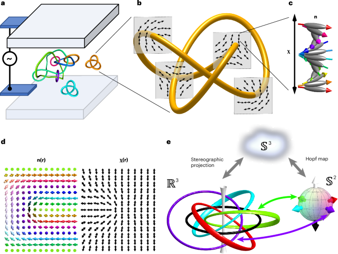
To resolve the detailed structure within heliknotons and fused heliknoton structures, we utilized a three-photon emission fluorescence polarizing microscopy setup, which is directly integrated with the IX-81 microscope described above. To prepare samples for three-photon emission fluorescence polarizing microscopy, after generating soliton structures in a cell with the polymerizable chiral LC mixture, ultraviolet light from a 20-W mercury lamp was concentrated onto a small region of interest through an aluminium foil mask with a pinhole to locally polymerize and preserve the orientational order by crosslinking the reactive mesogens. The small polymerization region allows heliknotons to be generated and ‘frozen’ at multiple spots within a cell sequentially, improving the throughput. Once polymerized, the cell was split apart and most of the unpolymerized 5CB molecules were washed away with isopropyl alcohol and replaced with index-matching immersion oil. This procedure was done to minimize birefringence of the LC material, which can lead to imaging artifacts, and maintain the LC \({\bf{n}}\left({\bf{r}}\right)\) configurations. A Ti-sapphire oscillator (Chameleon Ultra II, Coherent) operating at 870 nm with 140-fs pulses at 80-MHz repetition rate was used to excite the remaining 5CB molecules by three-photon absorption. The fluorescence signal is filtered with a 417/60-nm bandpass filter and detected in the forward-detection mode using a photomultiplier tube (H5784-20, Hamamatsu). The signal intensity of the three-photon absorption process scales with \({\cos }^{6}\left(\beta \right)\), where β is the relative angle between the long axis of the 5CB molecule and the polarization vector of light. For imaging scans done in this work, circularly polarized light, obtained by a quarter-wave plate, was utilized to extract the preimages of \({\bf{n}}\left({\bf{r}}\right)\) aligned along the far-field helical axis χ0, corresponding to regions with the lowest fluorescence signal. Isosurfaces extracted from experimental imaging were then analysed and contrasted with the corresponding numerical structure relaxed from initial conditions matching the experimental starting configuration.
Numerical modelling of heliknotons via energy minimization
Numerical modelling of fusion and fission of heliknotons and other knotted solitonic structures is based on minimizing the Frank–Oseen free-energy functional:
$$F\left[{\bf{n}}\left({\bf{r}}\right)\right]={F}_{\text{elastic}}\left[{\bf{n}}\left({\bf{r}}\right)\right]+{F}_{\text{electric}}\left[{\bf{n}}\left({\bf{r}}\right)\right]$$
(2)
via the finite-difference method. Here \({F}_{\text{elastic}}\) accounts for elastic energy penalties incurred due to splay (\({k}_{11}\)), twist (\({k}_{22}\)), bend (\({k}_{33}\)) and saddle-splay (\({k}_{24}\)) deformations and takes the form
$$\begin{array}{ll}{F}_{\mathrm{elastic}}[{\bf{n}}({\bf{r}})] \, = \, {\displaystyle{\int}} {{\mathrm{d}}}^{3}{\bf{r}}\left\{\frac{{k}_{11}}{2}{(\nabla \cdot {\bf{n}})}^{2}+\frac{{k}_{22}}{2}{[{\bf{n}}\cdot (\nabla \times {\bf{n}})+2\pi /p]}^{2}\right.\\\left.\qquad\qquad\qquad\,+\frac{{k}_{33}}{2}{[{\bf{n}}\times (\nabla \times {\bf{n}})]}^{2}-\frac{{k}_{24}}{2}\nabla \cdot [{\bf{n}}(\nabla \cdot {\bf{n}})+{\bf{n}}\times (\nabla \times {\bf{n}})]\right\}.\end{array}$$
(3)
The saddle-splay energy contributes to the energetics of defects and surface-anchoring energy53,54. Since the n(r) configurations considered in this work are continuous and strong anchoring conditions are applied, we set \({k}_{24}\) to zero. The other elastic constants \({k}_{11}\) (6.4 pN), \({k}_{22}\) (3.0 pN) and \({k}_{33}\) (10.0 pN) take the experimentally determined values of 5CB. Similarly, the electric contribution is defined by
$${F}_{\mathrm{electric}}[{\bf{n}}({\bf{r}})]=-\frac{1}{2}{\varepsilon }_{0}\int {{\rm{d}}}^{3}{\bf{r}}[{\varepsilon }_{\perp }{{\bf{E}}}^{{\bf{2}}}+\Delta \varepsilon {({\bf{n}}\cdot {\bf{E}})}^{2}],$$
(4)
where \({\bf{E}}\) is the applied field, \({\varepsilon }_{0}=8.854\times {10}^{-12}\,\text{F}\,{\text{m}}^{-1}\) is the permittivity of vacuum, \({\varepsilon }_{\perp }\) is the dielectric coefficient perpendicular to the director axis and \(\Delta \varepsilon\) is the dielectric anisotropy of the LC medium. For 5CB, \(\Delta \varepsilon\) and \({\varepsilon }_{\perp }\) take the values of 13.8 and 5.2, respectively. The equations of motion for the director field were obtained by varying the total energy functional and replacing the derivatives with their fourth-order finite-difference counterparts. This, subsequently, yields a set of coupled algebraic equations at each grid point to locally update the director field. To ensure numerical stability, an under-relaxation routine was performed such that the successive numerical solution is a weighted average of the old and new solutions: \({n}_{\mathrm{i}}\to \alpha {n}_{\mathrm{i}}+\left(1-\alpha \right){n}_{\mathrm{i}}^{{\prime} }\). The parameter \(\alpha \in \left[\mathrm{0,1}\right]\) is generally set to \(\alpha =0.1\) and was chosen empirically to ensure a convergent solution. To account for local distortions in the electric field due to the dielectric nature of the LC material, after each subsequent update for the director field, the voltage is updated by minimizing the free energy with respect to the electric field and substituting the derivatives of voltage with fourth-order finite-difference derivatives. This yields an equation to update the electric field at each grid point evolving the voltage simultaneously as the director field is relaxed. Periodic boundaries were assigned to the planes perpendicular to the helical axis, whereas hard boundary conditions were defined on the top and bottom of the cell. High-throughput grid calculations were performed in parallel via code written in C++ with CUDA acceleration.
Heliknotons are initialized from the ansatz6,9,17
$${{\bf{n}}}^{{\prime} }\left({\bf{r}}\right)={\bf{q}}{\left({\bf{r}}\right)}^{-1}{\vec{{\bf{N}}}}_{\mathrm{bg}}\left({\bf{r}}\right){\bf{q}}\left({\bf{r}}\right),$$
(5)
where \({\vec{{\bf{N}}}}_{{\mathrm{bg}}}\left(\vec{{\bf{r}}}\right)=\cos \left(2{{\pi}}z/p\right)\hat{{\bf{x}}}+\sin \left(2{\pi}z/p\right)\hat{{\bf{y}}}\) defines the background helical director field, \(p\) is the pitch and \({\bf{q}}\left({\bf{r}}\right)=\cos \left({\pi}{Qr}/p\right)+\sin \left({\pi}{Qr}/p\right)\hat{{\bf{r}}}\) is a quaternion. Here Q is an integer that defines the charge of the heliknoton and is set to unity for elementary heliknotons. In our modelling, to obtain the final heliknoton ansatz \({\bf{n}}\left({\bf{r}}\right)\), the z component of \({\bf{n}}\left({\bf{r}}\right)\) is inverted:
$${n}_{\mathrm{x}}={n}_{\mathrm{x}}^{{\prime} },\,\,\,\,\,\,\,{n}_{\mathrm{y}}={n}_{\mathrm{y}}^{{\prime} },\,\,\,\,\,\,\,{n}_{\mathrm{z}}=-{n}_{\mathrm{z}}^{{\prime} }.$$
(6)
For initial conditions involving multiple elementary heliknotons, a cut-off radius is chosen to be the pitch \(p\) to allow for the embedding of multiple heliknotons in a uniform helical background. This is carried out by superimposing the ansatz configurations for heliknotons localized at different locations \(\{{{\bf{r}}}_{\mathrm{i}}\}\). The ansatz above is then relaxed according to the energy-minimizing procedure described above.
To calibrate the elapsed time in simulations to match that of the experiments, we reconstruct the same initial conditions for both experiment and numerical simulations of the reconnection corresponding to Fig. 3 and Extended Data Fig. 6. For a node density of 253p−3, we find the time elapsed for each iteration to be 0.205 ms.
Fusion and fission response times
We explore the dynamic characteristics of elementary heliknotons fusing and splitting apart by pulsing the applied voltage. Here we describe the dependence of the response times \({\tau }_{{\mathrm{a}}}\) (\({\tau }_{{\mathrm{o}}}\)) as a function of the voltage amplitude in detail. Although a complete characterization of the switching dynamics is beyond the scope of this work, the most relevant parameter allowing one to tune the switching dynamics is the applied voltage magnitude (Extended Data Fig. 7). Given a pair of heliknotons in the trefoil state just before (after) a fusion event, the response time \({\tau }_{{\mathrm{a}}}\) (\({\tau }_{{\mathrm{o}}}\)) diverges for a critical voltage dependent on the separation distance and the relative orientation of the heliknoton–heliknoton pair. This critical voltage can be interpreted as the voltage that typically stabilizes a four-valent intermediate graph topology instead of completing the reconnection event. As the applied voltage deviates from the critical voltage, the response times sharply drop and saturate to finite subsecond values. Note that the response times in Extended Data Fig. 7 are somewhat smaller than those observed in Fig. 5b,c due to the closer distance at which the heliknotons were initialized in this context. The set of parameters used above can be translated to other experimental geometries by noting the Frank–Oseen free-energy functional can be rescaled by the pitch without influencing the equations of motion. Thus, the response time (neglecting initial conditions) appears to depend only on the dimensionless electric field defined by \(\widetilde{{\mathrm{E}}}=\sqrt{{\varepsilon }_{0}\Delta \varepsilon /\bar{K}}\left(V/\widetilde{{\mathrm{d}}}\right)\), where \(\widetilde{{\mathrm{d}}}\) is the thickness of the cell expressed in units of pitch \(p\) and \(\bar{K}\) is the average elastic constant at room temperature.
Visualization and topological characterization of heliknotons
The helical axis field \({\bf{\chi }}({\bf{r}})\) is obtained by constructing the chirality tensor \({C}_{\mathrm{ij}}={\partial }_{\mathrm{i}}{n}_{l}{\epsilon }_{\mathrm{jlk}}{n}_{\mathrm{k}}\), where Einstein summation convention is assumed and obtaining the dominant principal eigenvector, which defines the orientation of the local non-polar helical axis \({\bf{\chi }}({\bf{r}})\). Local regions within heliknotons that do not have a well-defined chiral axis correspond to vortex lines. In this work, we colour these vortex lines according to their local director orientation on the \({{\mathbb{S}}}^{2}\) sphere. Vortex knots obtained by sampling the raw grid points are often coarse. To improve the quality of these knots, vortices are first smoothed via Taubin smoothing to ensure a faithful reconstruction of the knot topologies55. These smoothed isosurface data are then used to construct a graph, which is traversed to find link components before and after knot reconnections. When graphs can be successfully resolved into links, the corresponding knot diagrams are imported into the KnotPlot freeware52 for three-dimensional visualization, after which they can further analysed. Ribbons of splay–bend in a tubular neighbourhood about the vortex lines are produced by constructing a tensor \({\mathbb{Q}}\left({\bf{\chi }}\right)={\bf{\chi }}\otimes {\bf{\chi }}-1/3\) and calculating the splay–bend parameter \({S}_{\text{SB}}={\partial }_{\mathrm{i}}{\partial }_{\mathrm{j}}{{\mathbb{Q}}}_{\mathrm{ij}}\) (here Einstein summation is assumed)56. The blue and yellow ribbons indicate regions with \({S}_{\text{SB}} > 0\) and \({S}_{\text{SB}} < 0\), respectively, and correspond to isosurfaces of \({S}_{\text{SB}}\) values of 10% of the average positive splay–bend \(\left\langle {S}_{\text{SB}}^{+}\right\rangle\) and 10% of the average negative splay–bend \(\left\langle {S}_{\text{SB}}^{-}\right\rangle\) within the tubular neighbourhood of the vortex knot. To produce smooth ribbons close to the vortex cores in which \({\boldsymbol{\chi }}\) is ill-defined, \({S}_{\text{SB}}\) at each grid point is locally averaged with its nearest neighbours.
Hopf indices of elementary and hybridized heliknotons are numerically computed according to the following procedure described elsewhere38,46. First, we make the identification \({b}^{\mathrm{i}}={\epsilon }^{\mathrm{ijk}}{F}_{\mathrm{jk}}={\epsilon }^{\mathrm{ijk}}{\partial }_{\mathrm{j}}{{\mathrm{A}}}_{\mathrm{k}}\), allowing us to associate the quantity \({\bf{A}}\) with a vector potential of \({\bf{b}}={\pmb{\nabla }}{\bf{\times }}{\bf{A}}\). The Hopf index Q can then be written as \(Q=\frac{1}{64{{\mathrm{\pi }}}^{2}}\int {{\mathrm{d}}}^{3}{\bf{r}}({\bf{b}}\cdot {\bf{A}})\). It follows that on computing \({\boldsymbol{b}}\), the vector potential \({\bf{A}}\) is obtained from numerical integration and Q can be obtained. All numerical derivatives are performed with fourth-order accuracy, yielding Hopf indices that agree within numerical error with the number of heliknotons initialized. The Hopf charge may also be determined by counting the linking number of different vectorized preimages47. The north- and south-pole preimages correspond to the director orientations along χ0 or the z axis. These preimages can be numerically extracted by computing isosurfaces according to the condition \(\left|{\bf{n}}\left({\bf{r}}\right)-{{\bf{n}}}_{\mathrm{t}}\right| < \eta\), where \(\eta\) is a numerical tolerance set to 0.1 corresponding to a small neighbourhood of allowed vectorized \({\bf{n}}\left({\bf{r}}\right)\) orientations surrounding the target orientation \({{\bf{n}}}_{\mathrm{t}}\).
Simulated POM movies were generated by applying a simple Jones matrix approach. We begin with a homogeneous input vector \({{\bf{E}}}_{0}={\left(\begin{array}{cc}1 & 0\end{array}\right)}^{{\mathrm{T}}}\) representing linearly polarized light along the x axis of a given wavelength λ. Rays of light are assumed to propagate along the far-field helical axis χ0 (along the z axis) of the cell followed by a crossed polarizer aligned with the y axis. For a small LC volume of thickness \(\Delta z\) with the director aligned with the x axis, the corresponding Jones matrix is
$${J}_{0}=\left(\begin{array}{cc}{{\rm{e}}}^{{\mathrm{i}}{\delta }_{\mathrm{eff}}} & 0\\ 0 & {{\mathrm{e}}}^{{\mathrm{i}}{\delta }_{0}}\end{array}\right),$$
(7)
where \({\delta }_{0}=2{\pi}{n}_{\mathrm{o}}\Delta z/\lambda\) and \({\delta }_{\mathrm{eff}}=2{\pi}{n}_{\mathrm{eff}}\Delta z/\lambda\) are the phases of the fast and slow axes, respectively. The extraordinary (\({n}_{{\mathrm{e}}}\)) and ordinary (\({n}_{{\mathrm{o}}}\)) refractive indices are related to the effective refractive index accounting for the out-of-plane angle \(\theta\) of the director and is given by
$${n}_{{\mathrm{eff}}}=\frac{{n}_{\mathrm{o}}{n}_{{\mathrm{e}}}}{\sqrt{{\cos }^{2}\left(\theta \right){n}_{{\mathrm{e}}}^{2}+{\sin }^{2}\left(\theta\right){n}_{\mathrm{o}}^{2}}}.$$
(8)
In a medium of 5CB, \({n}_{{\mathrm{e}}}\) and \({n}_{{\mathrm{o}}}\) assume the values of 1.77 and 1.58, respectively. More generally, for directors with an angle \(\phi\) from the x axis in the x–y plane, a rotation \(R\left(\phi \right)\in \mathrm{SO}\left(2\right)\) can be applied to \({J}_{0}\) according to \(J\left({\theta},{\phi}\right)=R\left(\phi \right){J}_{0}\left({\theta }\right)R{\left(\phi \right)}^{{\mathrm{T}}}\). Applying this Jones matrix ansatz to the discretized grid geometry above, the effective Jones matrix for each point (x, y) in the focal plane is obtained by multiplying successive Jones matrices from different layers together corresponding to a column with \({N}_{\mathrm{z}}\) elements along the helical axis:
$$M(x,y)=\mathop{\prod }\limits_{1\le i\le {N}_{\mathrm{z}}}J(\theta (x,y,{z}_{\mathrm{i}}),\phi (x,y,{z}_{\mathrm{i}})).$$
(9)
The output polarization for a given wavelength is obtained by applying \(M\left(x,y\right)\) to the input polarization and selecting the second component \({{\mathrm{e}}}_{\mathrm{y}}^{\left({\lambda }\right)}\) due to the output polarizer. The normalized intensity is computed from the squared magnitude of the output. This procedure is carried out for 650-, 550- and 450-nm light, with relative intensities of 1.0, 0.6 and 0.3, respectively, determined by the spectral content of the light source used in the experiments. For still POMs, the open-source software Nemaktis57 with the ability to model more complex optical effects via ray-tracing and beam propagation (Extended Data Fig. 4b, bottom) was found yielding images generally consistent with the ones modelled by the Jones matrix approach. We found that both our Jones matrix approach and Nemaktis yield results that agree well with the experiments.
Tracking interactions between heliknotons via POM imaging
To track the separation vector between two heliknotons during fusion and fission using POM, we make use of their key property: heliknotons have orientations and positions along the far-field helical axis coupled, thereby undergoing a screw-like rotational motion when translated along the far-field helical axis10. In the POM video (Supplementary Video 2), by recording the change in a relative angle describing the heliknoton’s azimuthal orientation, the heliknoton’s dynamics across the sample thickness (along the z axis and far-field helical axis) can be tracked, in addition to tracking its lateral displacement. It follows that by defining \(\psi\) to be the relative angle between the long axes of the two heliknotons, one obtains \(\psi =2{\pi}{s}_{\mathrm{z}}/p\), where \({s}_{\mathrm{z}}\) is their separation in z. Since the in-plane heliknoton separation can be directly determined from the POM images, the full separation vector between the two heliknotons can be reconstructed. The same procedure can be applied to simulated POM images of numerically simulated heliknotons as well, to enable a direct comparison of fusion/fission between experiments and simulations. In experimental cells that are less than \(4p\) in thickness, heliknotons tend to persist in the midplane of the cell, allowing \(\psi\) to be easily determined as the heliknotons are perturbed from equilibrium by changing the voltage or laser tweezers manipulation.
Characterization of knot topology
A crucial aspect of our findings is the translation of our vortex knots, and the simplified diagrams introduced to faithfully represent their topologies and site-specific reconnections. We choose to represent these reconnections in diagrams via blue and green bands corresponding to band surgeries associated with internal and external heliknoton reconnections, respectively (Fig. 4 and Extended Data Fig. 9d–g). Additionally, information about the local winding number of the vortices is also important as reconnections often occur through a reconnection mechanism involving the annihilation (fusion) or pair creation (fission) between the vortex segments of opposite winding number. We find that for all links obtained, all reconnections analysed can be identified with the mathematical operation of coherent band surgery in which orientations are preserved3,45. From the diagrams produced, one can track the evolution of the writhe as vortex knots and links undergo reconnections3,42,43,44,45. The writhe serves as a simple measure of complexity in the knots we obtain as they are generated from right-handed trefoil building blocks in which the action of incorporating another trefoil into a complex composite knot only increases the writhe (Extended Data Fig. 9).
Like the writhe, one can compute the so-called reconnection number for a given knot or link. The reconnection number of a knot or link is the least number of reconnections that need to be performed to transform it to an unknot43,45. In general, this number is not known, but computable bounds on it from below exist (such as the so-called signature of the knot) and a very particular upper bound is always known that we shall call the R-number of the knot or link and denote by R(K), where K is the link. In this case, one simply smooths crossings such that the local knot orientation is preserved (Extended Data Fig. 9a)45. The circles generated by this action are called Seifert circles3,45. The R-number is defined as45
where \(c\) is the number of crossings in the original diagram and \(s\) is the number of Seifert circles. The meaning of the formula is that one can perform reconnections at \(R\) crossings (it is lower than the total number of crossings) and obtain an unknot45. This is shown in Extended Data Fig. 9b for the trefoil knot and implicitly for other examples in the figure. Once one has the reconnection numbers for a reconnection pathway (\(K_{\mathrm{i}}\to K_{\mathrm{f}}\)), it follows that the relative R-number \(\left|{R}(K_{\mathrm{i}})-{R}(K_{\mathrm{f}})\right|\) is a well-defined quantity that estimates from above the minimal number of reconnections necessary to transform \(K_{\mathrm{i}}\) to \(K_{\mathrm{f}}\). If the link K has all positive crossings (Extended Data Fig. 9), then R(K) is equal to the reconnection number of K. In general, for any K, the link or knot K can be transformed into an unknot in R(K) reconnections. R(K) is the least among all the possible unknottings when K is positive.