

In this section, we outline the method we used to assign genomes to each species cluster. We also verify the robustness of the species assignment by using three different methods and show that they give identical results.
Comparisons of genomes from bacterial populations often reveal clusters at different length and divergence scales (Jain et al., 2018). But the interpretation of such clusters is controversial (Cohan, 2002; Fraser et al., 2009). There are three main possible interpretations for such patterns. One interpretation is that the clusters represent the bacterial analog of eukaryotic species, which are sexually and ecologically isolated from each other. In practice, a whole-genome divergence cutoff of 5% is frequently used to define bacterial species (Jain et al., 2018). An alternative interpretation is that clusters are the result of clonal expansions of particular strains from a much more diverse and possibly more genetically homogeneous population. The third interpretation is that the clusters are the result of uneven sampling from a larger and more diverse population. The unique combination of having a large collection of genomes, with minimal compositional bias, from a geographically isolated population allows us to test these alternatives. We will mainly aim to distinguish between the first two interpretations and the third one by checking whether there are robust genomic clusters in our sample. More discussion on the evidence concerning the first two hypotheses can be found in Appendices 3 and 5.
We used three different methods to check whether the genomes form robust clusters: the phylogenetic tree of the 16S rRNA sequences, average genome-wide divergence from the two reference genomes OS-A and OS-B’, and patterns of divergences between triplets formed by the SAG and the two reference sequences at different loci. The phylogenetic tree of the 16S is the simplest and still the most commonly used method to characterize the diversity of natural microbial communities (Yarza et al., 2014). Because of its practical importance, we included it for comparison with the other two methods. However, in a highly recombining population like the Yellowstone Synechococcus, it is not clear to what extent the 16S divergence accurately reflects the whole-genome diversity. To address this question, we used the divergences across the entire genome as a comparison. The main limitation of using summary statistics such as the average divergence across the entire genome is that it obscures heterogeneities along the genome that could have important ecological and evolutionary implications. There are different ways to address this concern. Here, we used an extension of a method first used in Rosen et al., 2018, which provides a coarse description of the variation in the diversity patterns across different loci. We present the results from each of these analyses next.
We first constructed the phylogenetic tree of 16S sequences. Predicted 16S rRNA sequences (117 from 331 filtered SAGs) were extracted and aligned using MAFFT (v7.453) (Katoh and Standley, 2013). Two sequences (SAGs MA02M11_3 and MuA02C9) were incomplete and were removed from the analysis. The remaining (115) sequences were hierarchically clustered using the average linkage (UPGMA) method implemented in Scipy. Results are shown in Appendix 2—figure 3, with the colored background showing the species assignment using whole-genome divergences (see below) for comparison. We found perfect agreement between the whole-genome assignment and the largest three clusters in the 16S phylogenetic tree.
The average divergence within the α cluster is approximately half that of β (1⋅10−3 vs 2⋅10−3). However, a significant fraction of the average divergence within β was due to two outliers (MuA1L16 and MusA1J8). After removing the outliers, the average divergence within β decreased to 1.7⋅10−3. Closer investigation of the alignments revealed that both outlier β sequences contained a short segment of three SNPs that were identical to all α sequences and different from all other β sequences, at positions 1067–1072. In addition, MuA1L16 contained a larger segment of almost 200 bp (positions 390–570) containing 10 SNPs and an insertion that were different from all other β and were identical to the consensus α. Apart from these segments, the outlier sequences were typical of the β species. This pattern is similar to the SNP blocks discussed in the main text and in Appendix 6 and therefore is likely the result of hybridization between α and β.
We compared the 16S rRNA clusters to whole-genome divergences from the two reference genomes, OS-A and OS-B’. We aligned all of the predicted genes from each SAG to all of the coding DNA sequences (CDS) from each reference genome using BLAST (v2.13.0+) (Altschul et al., 1990). For each SAG, we calculated the divergence to each reference genome (d=1−pident/100) and calculated the average over the best hits across all genes. The results for all SAGs with more than 100 hits to both references are shown in Figure 1A. Three clear clusters were observed, which we labeled as α, β, and γ. The species of each SAG was assigned as the label corresponding to the cluster it belonged to in Figure 5A.
The previous two metrics do not reflect possible heterogeneity in the patterns of diversity along the genome. To characterize this variation on a gene-by-gene basis, we extended a method that was previously used to analyze amplicon data from the Mushroom Spring in Rosen et al., 2018. We refer to this method as gene triplet analysis. This analysis exploits the separation of scales between and within species clusters. At most loci and in most cells, we observed previously in order to coarse grain the high-dimensional matrix of pairwise divergences into a small number of discrete patterns. Specifically, we take triplets of sequences from the SAGs, OS-A, OS-B’, at loci where all three are homologous and calculate the divergences between all three pairs of sequences. These divergences typically form a triangle as shown in Appendix 2—figure 1. Note that it is possible to have triplets of divergences that violate the triangle inequality, which cannot be represented as triangles in a two-dimensional space. In our data, such cases were rare, but this may not be generally true, particularly for sequences that are not clearly separated and which are the result of extensive recombination. Note, however, that the classification into distinct patterns given below can still be done even in these cases. To reduce the dimensionality of the data further, we define a main cloud diameter dM=0.1 for the diversity within species. We then classify the shape of the triangle into the 5 distinct patterns shown in Appendix 2—figure 1, depending on whether each side of the triangle is longer or shorter than dM. For example, denote the divergence triplet by (dXA,dXB,dAB), representing the divergences between the SAG sequence and OS-A, the SAG sequence and OS-B’, and OS-A and OS-B’, respectively. Then the first pattern in Appendix 2—figure 1A (labeled ‘XA–B’) contains loci where dXA<dM, dXB≥dM, and dAB<dM, the second pattern (labeled ‘XAB’) contains loci where dXA<dM, dXB<dM, and dAB<dM, and so on. The cutoff of dM=0.1 is the same as the one used in Rosen et al., 2018 and provides a good separation between species at a gene by gene basis. The results of our analysis, however, do not depend on the specific value of dM as discussed at the end.
For each SAG, we assigned all genes that were orthologous to OS-A and OS-B’ to one of the five patterns described above. The three rows in Appendix 2—figure 1 show typical examples of an α (Appendix 2—figure 1A), a β (Appendix 2—figure 1B), and the γ (Appendix 2—figure 1C) SAG. The majority of genes across each row in Appendix 2—figure 1 are found in the XA–B, XB–A, and X–A–B patterns, respectively. This is consistent with the species clusters we saw in the genome-wide average divergences from before. However, we also find a significant minority of genes forming other patterns, most notably XAB, representing genes where all three sequences are within the main cloud (d<dM). Some of these genes were contained in the divergence troughs discussed in the main text. In the case of the γ SAG, the fact that X–A–B is the dominant pattern rules out the possibility that γ is a hybrid resulting from the mixture of α and β. Such hybrids have been observed after recent clonal expansions in acid mine drainage microbial communities (Tyson et al., 2004; Lo et al., 2007), but do not appear to be present at substantial frequency in the Yellowstone community. Instead, it appears that γ is a distinct species that diverged from the other two around the same time α and β diverged from each other.
Using the pattern described above allows us to compare different SAGs to each other and allows us to test the robustness of the species assignment based on the average genome-wide divergence. Specifically, we assigned to each SAG a gene triple fingerprint f=(fXA−B,fXAB,fX−A−B,fX−AB,fXB−A), representing the fraction of genes with each pattern (note that ∑ifi=1). We then compared the fingerprints of each SAG with the species assignment based on the average divergence from OS-A and OS-B’ from Figure 1A. We found that the fingerprints formed three clear patterns that exactly matched the assignments based on the average divergence (Appendix 2—figure 2). We tested this assignment for different values of dM ranging from 1% to 20% and found that the fingerprint patterns were robust across the entire range (data not shown). These results show that the classification into distinct species is robust and consistent across the three methods described.
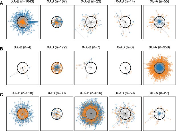
Species clusters at the gene level approximately match those at the genome level.
Figures show gene-by-gene comparison of three cells to the OS-A and OS-B’ reference genomes. The cells shown are representative of the α (A; OctA1J9) and β (B; MA02H14_2) clusters and the one γ cell (C; OcA3L13). Each core gene with homologs in both OS-A and OS-B’ was compared to the references and the divergences plotted as a triangle with each side length equal to the divergence between a given pair. The cell sequence is represented by a black dot, with the OS-A and OS-B’ sequences represented by the orange upward and blue downward triangles, respectively. The black circle is a 10% radius which was chosen as a cutoff to classify each gene. The different columns show genes in one of the five possible patterns labeled as follows: XA–B (the cell sequence is less than 10% diverged from OS-A and more than 10% diverged from OS-B’), XAB (all three sequences are within 10% of each other), X–A–B (all three sequences are more than 10% diverged from each other), X–AB (the cell is more than 10% diverged from both OS-A and OS-B’, but both references are less than 10% diverged from each other), and XB–A (the cell is less than 10% diverged from OS-B’ and more than 10% diverged from OS-A).
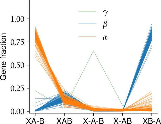
The proportion of gene triplet patterns shows three distinct clusters.
The proportion of genes in each of the five patterns shown in Appendix 2—figure 1 is shown for each cell passing our quality control criteria (see Appendix A). Lines represent different cells and are colored according to the species classification based on whole-genome divergences.
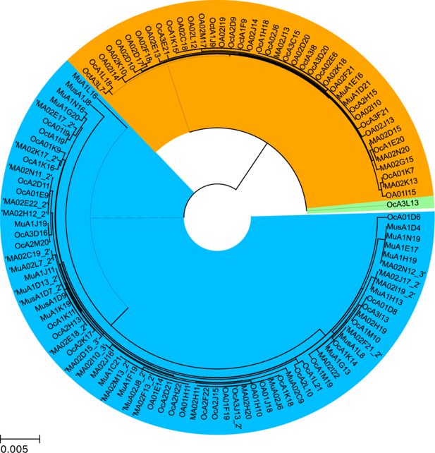
Phylogenetic tree inferred from 16S rRNA agrees with whole-genome species classification.
The pairwise divergences between all 16S sequences passing quality control were calculated from the multiple sequence alignment performed using MAFFT (Katoh and Standley, 2013). The tree was generated using a hierarchical agglomerative clustering algorithm with average linkage (UPGMA) as implemented in SciPy (Virtanen et al., 2020).