
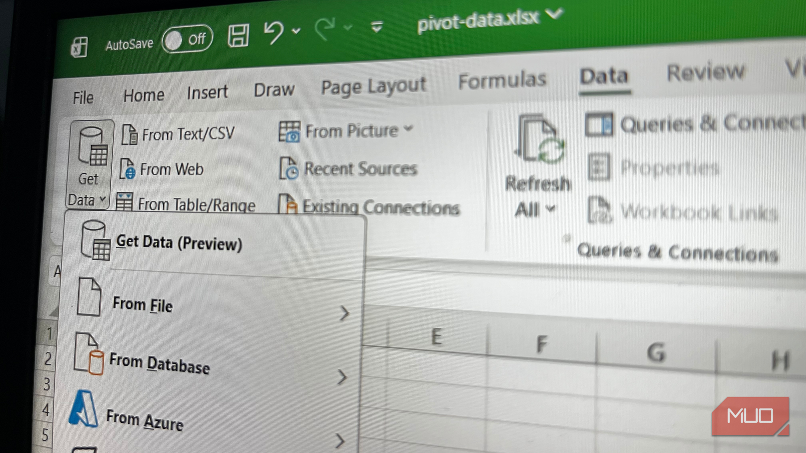
Most people set up a dropdown list to make spreadsheets smarter with Excel’s data validation. However, the Custom option in the Data Validation dialog accepts any formula that returns TRUE or FALSE, which means you can enforce rules that dropdowns were not built to handle.
Duplicate prevention, text pattern requirements, date restrictions, and calculated limits all run through one setting that most people skip right past. Here’s how I use custom formulas to lock down my spreadsheets properly.
Related
Excel’s SEQUENCE function made me realize I’d been wasting time manually filling date columns
It replaced my date-filling workflow, and I’m not going back.
Custom formulas let you control far more than a list
The Custom option accepts any TRUE/FALSE formula as a validation rule
Excel’s data validation has several built-in options such as whole numbers, decimals, dates, text length, and, of course, dropdown lists — it’s one of those Excel tricks worth learning early. These cover common scenarios, but they’re rigid. The moment you need a rule that doesn’t fit neatly into one of those categories, you’re stuck. That’s where the Custom option comes in.
It lets you write a formula that evaluates to TRUE or FALSE. If the formula returns TRUE, Excel accepts the entry. If it returns FALSE, the entry gets rejected. Here’s how to set it up:
Select the cell or range you want to validate.
Go to the Data tab and click Data Validation.
Under Allow, select Custom.
Enter your formula in the Formula field.
Click the Error Alert tab and write a clear message explaining why an entry might be rejected.
Click OK.
Remember that when applying validation to a range, your formula should reference the first cell in that range. Excel automatically adjusts the reference for the remaining cells, just like it does when you drag a formula down. If you get this wrong, your validation will either not work or apply the same check to every cell regardless of position.
Any formula that produces a TRUE/FALSE result works — COUNTIF, AND, OR, LEN, LEFT, ISNUMBER, or even nested combinations. If you can write it in a cell, you can use it as a validation rule.
Prevent duplicate entries with a COUNTIF formula
It flags repeats before they cause problems
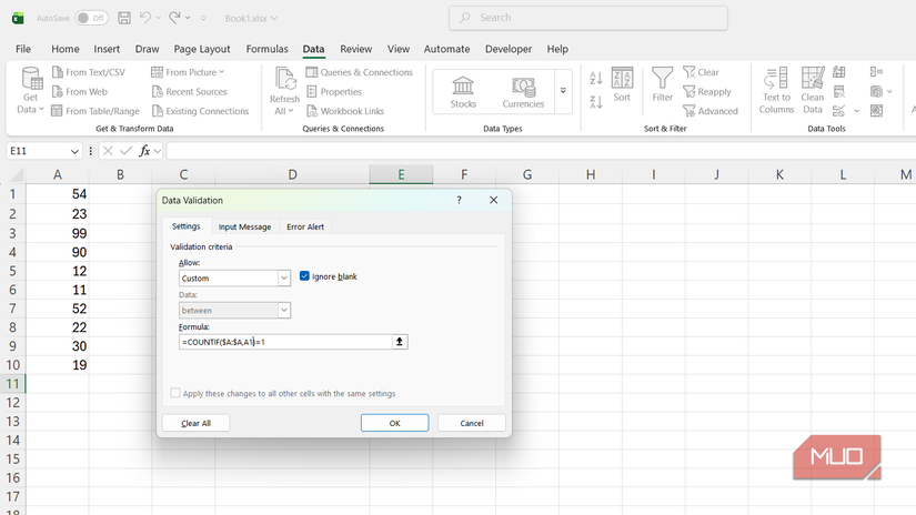
Screenshot by Yasir Mahmood
Duplicates are one of the most common data entry mistakes, and they’re annoying to clean up after the fact. Employee IDs, invoice numbers, and email addresses shouldn’t appear twice in the same column. Instead of scanning for duplicates manually, trying to highlight duplicates in Excel after the fact, or running a cleanup later, you can stop them at the point of entry.
You can use the following formula:
=COUNTIF($A:$A,A1)=1
This counts how many times the value in A1 appears in column A. If it appears exactly once, the entry is valid. If COUNTIF returns a value greater than 1, it means a duplicate already exists, and Excel blocks it.
For example, say you’re tracking order IDs in column A. You enter “ORD-1042” in A2, and it’s accepted because it’s the first instance. If someone tries entering “ORD-1042” again in A10, the validation kicks in and rejects it.
Using $A:$A as the range works fine for smaller datasets, but it forces Excel to scan the entire column. If you’re working with thousands of rows, narrowing the range to something like $A$2:$A$500 improves performance. It’s a small adjustment, but it matters on larger spreadsheets.
Force entries to follow a specific pattern or length
LEN and LEFT keep the data consistent
Inconsistent entries are a quiet problem. Someone types a 5-character product code where it should be 8, or skips the required prefix, and now your filter breaks downstream. Custom validation can enforce both length and pattern in one rule. For length, you can use the following formula:
=LEN(A2)=8
This rejects anything that isn’t exactly 8 characters. For a required prefix, use LEFT:
=LEFT(A2,3)=”PRD”
You can combine both conditions with AND to enforce them simultaneously:
=AND(LEN(A2)=8,LEFT(A2,3)=”PRD”)
For example, if your inventory system uses codes like “PRD-1047”, always 8 characters, always starting with “PRD”, then this formula ensures every entry follows that structure. Type “PRD-1047” and it’s accepted. Type “PR-1047” or “INV-1047” and Excel rejects it on the spot.
This is useful when multiple people work on the same spreadsheet. You can’t always control how carefully someone reads the formatting instructions, but you can make sure Excel enforces them regardless.
Restrict dates so no one enters anything in the past
TODAY() keeps your date entries forward-looking
A past date in a deadline or delivery column is almost always a mistake. Rather than catching these errors during review, you can block them outright with a simple formula:
=A2>=TODAY()
This ensures every date entered is either today or in the future. Since TODAY() recalculates automatically, the validation stays current without any manual updates. You can go further by restricting entries to a specific window. For example, if you only want dates within the next 30 days:
=AND(A2>=TODAY(),A2<=TODAY()+30)
This proves handy for scheduling forms where someone booking a meeting three months out would be just as wrong as entering yesterday’s date.
This validation only checks the entry at the time it’s typed. If someone enters tomorrow’s date today, it won’t retroactively flag it as invalid once that date passes. For that, you’d need conditional formatting as a secondary check.
These rules get stronger when you combine them
Stack multiple conditions for tighter control
Most examples covered here use a single condition, but AND and OR let you layer multiple checks into one formula. You could validate that a cell contains a future date, falls within budget, and follows a naming convention — all in a single rule. Pair that with custom error messages that explain exactly what went wrong, and you’ve built a spreadsheet that practically trains people to enter data correctly. From here, adding conditional formatting to visually flag borderline entries could be the next step.