
Single-shot readout
We investigate individual Ti atoms on the oxygen binding site of an MgO/Ag(100) substrate (see “Methods”), which have been shown to carry an electron spin S = 1/2 that can be ESR driven by an RF voltage at the STM junction16, in an external magnetic field oriented out-of-plane. Ti has different isotopes carrying nuclear spins 0, 5/2, or 7/2. In particular, 49Ti has nuclear spin I = 7/2 and couples to the electron spin with an out-of-plane hyperfine coupling component A⊥ = 130 MHz28, resulting in a total of 16 energy levels (Fig. 1a). The hyperfine coupling causes a shift in the ESR transition frequency that depends on the nuclear spin state, which is absent for Ti isotopes with I = 0 (Fig. 1b, c). The observation of multiple ESR peaks in a single sweep indicates that the nuclear spin state changes much faster than the averaging time of 3 s for each datapoint under conventional ESR settings. The peak heights are a measure of the population distribution of the various nuclear spin states: the nuclear spin resides longer in the mI = −7/2 state as a result of nuclear spin pumping by inelastic electron scattering27,28, where mI refers to the magnetic quantum number of the nuclear spin along the external magnetic field Bz. Being a time-averaged measurement, however, the ESR frequency sweep does not provide information on nuclear spin transition timescales.
Fig. 1: Time-resolved switching of the nuclear spin state.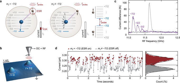
a Diagram of the measurement scheme: the I = 7/2 nuclear spin (blue) of a 49Ti atom coupled to the S = 1/2 electron spin (brown) via the hyperfine interaction. Only when the nuclear spin is in the mI = −7/2 state, does the applied RF signal at frequency fprobe lead to a tunneling current increase IESR. Right: spin energy diagram in the limit of a strong magnetic field, where the Zeeman splitting dominates and the eigenstates can be approximated by product states. b STM topography (10 pA, 60 mV) of two Ti isotopes on MgO/Ag(100). c ESR frequency sweeps (3.0 pA, 60 mV, Bz = 1.35 T, VRF = 17 mV, averaging time 3 s, lock-in frequency 270 Hz) measured on the two Ti atoms in (b). VRF refers to the zero-to-peak RF voltage amplitude at the tunnel junction. d Section of a time trace of the tunneling current at fixed tip height (60 mV, averaging time 20 ms) with fprobe corresponding to mI = −7/2. The current histogram on the right is fitted with a two-Gaussian distribution (black line).
In order to resolve changes between the nuclear spin states, we measured the ESR signal in the time domain instead of in the frequency domain. We switched off the STM feedback loop and sent a continuous RF signal to the tunneling junction with a fixed frequency fprobe, resonant with a transition of the electron spin magnetic quantum number mS between states |mS,mI〉 = |↓, −7/2〉 and |↑, −7/2〉, resulting in an additional ESR current IESR only when mI = −7/2, as illustrated in Fig. 1a. Figure 1d shows the current measured for several seconds, revealing stochastic switching between two discrete levels. The two levels become apparent in a histogram of the time trace as two Gaussian distributions separated by a current offset. In contrast, when we use an off-resonance frequency, the current is distributed as a single Gaussian (Supplementary Fig. 1a). We also performed reference measurements on a Ti isotope with I = 0 (Supplementary Fig. 1b, c), each revealing a single Gaussian distribution as well. We thus attribute the observed switching to quantum jumps between the probed state (mI = −7/2) and any of the other seven nuclear spin states (mI ≠ −7/2).
Since the observed switching time is considerably longer than the averaging time (20 ms), the majority of datapoints constitute a single-shot readout of the nuclear spin. Note that the nuclear spin state is projected at a singular event sometime during the averaging time by an electron passing the adatom. The state is then read out repeatedly during the remaining time to integrate the current to reach a measurable signal strength. This is possible because, in the product state limit, reading out the electron spin state mostly leaves the nuclear spin unchanged after projection. We achieve readout fidelities of up to 98% for both the probed state being occupied and it being unoccupied (see Supplementary Information).
We can probe different nuclear spin states without changing fprobe by adjusting the height of the magnetized probe tip, which exerts an additional magnetic field on the atom29. As we adjust the tip height (i.e., setpoint current), different values of mI become resonant with fprobe (Fig. 2a). We measured current time traces at different tip heights (i.e., different total fields), resulting in a set of current histograms plotted together in Fig. 2b–f. Within the sweep range of the setpoint current, the histograms are found to feature a bimodal distribution in three windows around 3.2, 2.8, and 2.4 pA, matching the resonances of the nuclear spin states mI = −7/2, −5/2, and −3/2, respectively. While for mI = −7/2 the distribution is ~50–50 (Fig. 2e, f), the other states are found to be occupied much less than half of the time (Fig. 2c).
Fig. 2: Readout of different nuclear spin states.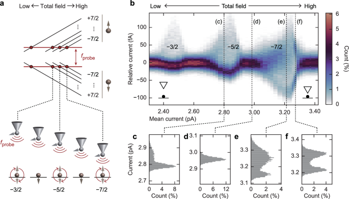
a Energy diagram of the spin states as a function of magnetic field (top) and schematic of the experiment shown in (b), indicating that at certain tip heights fprobe matches the Zeeman splitting corresponding to one of ml states (bottom). b Color map of current histograms similar to Fig. 1d for different heights of the magnetic STM tip (bias voltage 60 mV). The horizontal axis represents the mean current for each time trace, which is a measure of the total magnetic field. c–f Current histograms, corresponding to the labeled vertical dashed lines in (b).
Lifetime of the nuclear spin
Analysis of the time traces enables us to extract the dwell times of the nuclear spin states. We label each point in the time trace as either in the probed state or not, using a threshold determined by the intersection point of the two Gaussian distributions (Fig. 1d). We measure individual dwell times tdwell for each occurrence of consecutive time spent in the probed state (Fig. 3a). Using an exponential fit, we find a lifetime T1CW of about 100 ms for mI = −7/2 (Fig. 3a). We note that this is the nuclear spin lifetime under continuous-wave (CW) ESR driving and readout by the tunneling current.
Fig. 3: Dwell time of different nuclear spin states.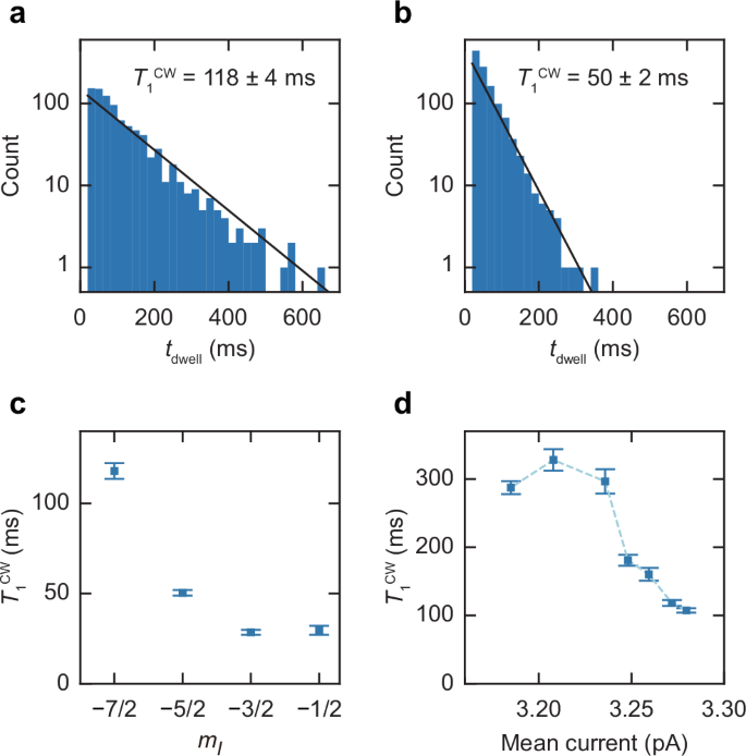
a, b Histograms of the distribution of the individual dwell times tdwell of mI = −7/2 and mI = −5/2, respectively. Fitting with an exponential function gives the characteristic dwell time T1CW. Error bars of T1CW are the standard deviations in the exponential fit parameter. c T1CW for mI = −7/2, −5/2, −3/2, −1/2, applying corresponding fprobe at the same tip height. d T1CW of mI = −7/2 at different tip heights around the resonance point.
To compare T1CW between different nuclear spin states, we repeated the experiment for different fprobe values while leaving the tip height unchanged to avoid variations in current-induced nuclear spin pumping (Fig. 3b, c, see also Supplementary Fig. 2). We observe that for fprobe being resonant with any of the mI ≠ −7/2 transitions, T1CW is significantly shorter than for mI = −7/2. This may be partly attributed to the fact that selection rules allow these states to transition in both directions (ΔmI = ±1), whereas the mI = −7/2 state can only switch to mI = −5/2 (ΔmI = +1). In addition, these experiments were performed in the presence of a spin-polarized current which constantly excites the system towards mI = −7/2.
However, neither of the above arguments can explain the fact that T1CW keeps decreasing beyond mI = −5/2, suggesting that the spin pumping efficiency depends on the nuclear spin state. We believe this may be because the hybridization between neighboring spin states depends on mI directly, which derives from the Clebsch-Gordan coefficients (see Supplementary Table 1). In addition, Fig. 3d shows how T1CW changes as we vary the tip height around the resonance point for mI = −7/2. We find that T1CW is increasing further up to ~300 ms as the system is detuned from resonance. This implies that the continuous ESR driving of the electron spin may affect T1CW as well.
In order to find the intrinsic lifetime T1 of the undisturbed nuclear spin and to identify its limiting relaxation mechanisms, we applied a pulsed readout scheme illustrated in Fig. 4a (see “Methods”). Here, we set the voltage (both DC and RF) to zero in between pulses. The probe pulses consisted of similar DC + RF conditions as in the continuous-wave experiments mentioned above. We set the tip height such that fprobe matches the resonance frequency for mI = −7/2. As shown in Fig. 4b, the voltage pulses lead to sharp peaks in the current, each of which we can assign either the value 1 (for mI = −7/2) or 0 (mI ≠ −7/2), using a threshold as introduced in Fig. 1d. For each pair of probe pulses A and B, there are four possible event scenarios, resulting in conditional probabilities P(B|A) (Fig. 4c, d).
Fig. 4: Intrinsic nuclear spin lifetime with pulsed detection scheme.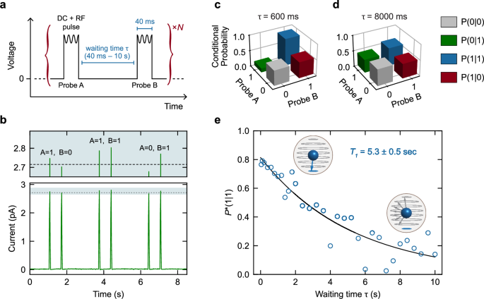
a Schematic of the pulse measurement scheme. One detection event consists of two probe pulses, with a variable waiting time τ in between, with zero bias voltage. Each probe pulse consists of a DC voltage (70 mV) and an RF signal at fprobe = 12.75 GHz, corresponding to mI = −7/2 (Bz = 1.6 T, VRF = 22.6 mV). For each τ, we repeat between N = 443 and N = 704 detection events. b Bottom: section of a measured current time trace (τ = 600 ms) showcasing three detection events. Top: zoom on the shaded area. For each event, the current of the probe pulses A and B indicates whether mI = −7/2 (1) or not (0), based on the current threshold (dashed line) determined from a histogram of all probe pulses. c, d Conditional probabilities P(B|A) for τ = 600 ms and τ = 8000 ms, respectively. e Corrected conditional probability P*(1|1) as a function of τ. P*(1|1) represents the intrinsic decay of the nuclear spin. An exponential fit (Ae−τ/T1, black curve) gives the intrinsic lifetime T1 of the mI = −7/2 nuclear spin state (T1 = 5.3 ± 0.5 s, A = 0.81 ± 0.03).
By changing the waiting time τ between the pulses, we then find the conditional probability as a function of τ (Fig. 4e). We take the unintentional pumping of the nuclear spin by the second probe pulse into account, correcting P(1|1) to P*(1|1) = [P(1|1)−P(1|0)]/[1−P(1|0)] (see Supplementary Information). P*(1|1)(τ) is expected to decrease exponentially as a function of τ due to relaxation processes at a timescale of T1. By fitting with an exponential function, we obtain T1 = 5.3 ± 0.5 s for mI = −7/2. Similar measurements on an identical 49Ti atom yielded a value of T1 = 4.3 ± 0.8 s (Supplementary Fig. 3). This T1 is seven orders of magnitude larger than the lifetime of the electron spin in the same atom (~100 ns)16. In addition, the extracted lifetime is an order of magnitude larger than T1CW measured in the continuous-wave experiment (Figs. 1 and 2), confirming the hypothesis that the nuclear spin state is affected by continuous ESR driving and DC readout.
Relaxation mechanism
To develop an understanding of how DC spin pumping and ESR driving affect the nuclear spin, we repeat the pulsed experiment introduced in Fig. 4, but now with additional voltages in the waiting time to investigate perturbation of the nuclear spin (Fig. 5a–c) (see “Methods”). In a first variant, we add a DC bias voltage during the waiting phase and fix the waiting time to 2 s. The figure of merit is P(1|1), now left uncorrected by P(1|0) as we intentionally disturb nuclear spins during the waiting time (see Supplementary Information). In Fig. 5a, we plot P(1|1) against the bias voltage in the waiting phase. P(1|1) is found to increase with positive voltage, whereas it decreases with negative voltage.
Fig. 5: DC or RF in the waiting period.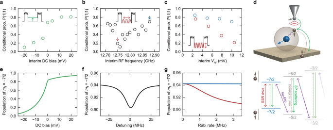
a Conditional probability P(1|1) as a function of DC voltage during the waiting section between the two probe pulses (see inset schematic), with a fixed waiting time τ = 2 s. b P(1|1) as a function of RF frequency in the waiting section (τ = 600 ms, VRF = 10.4 ± 0.3 mV). c Conditional probability P(1|1) as a function of RF voltage amplitude in the waiting section (interim VRF), for two different frequencies highlighted in (b) (red: on-resonance frequency, blue: off-resonance frequency). d Schematic of the possible transition dynamics between spin states: spin resonance drive of the electron spin (red), flip-flop quantum jump between nuclear and electronic spins mediated by hyperfine coupling (purple), environmental scattering of electronic spin (gray, dashed), electron spin scattering via spin-polarized STM tip (green). e–g Rate equation simulations of the experiments performed in (a), (b), and (c), respectively. The model includes all processes indicated in (d) and implements them as transition rates between eigenstates. The populations are recorded after time evolution from the initial state |↓, −7/2〉. Since the simulation does not quantitatively reproduce the experimental unperturbed nuclear lifetime, we chose simulated evolution times to be the same fraction of the simulated lifetime as the experimental ratio τ/T1 to capture a comparable moment in the decay process (see Supplementary Information).
We attribute this to dynamic nuclear spin polarization resulting from electron spin pumping, which is a combination of two processes depicted in Fig. 5d: flip-flop quantum jumps between a nuclear and electron spin due to hybridization as a result of the hyperfine coupling, and inelastic electron scattering. The former can happen both ways, while the latter is favored in one direction due to the spin polarization of the tip. As a result, the two processes together pump the system towards mI = −7/2 or mI = +7/2, depending on the voltage polarity27,28.
We note that, since Ti on the oxygen binding site displays a continuous-wave ESR signal only for positive voltages30, it was previously not possible to observe nuclear spin pumping at negative bias voltage. With our pulsed readout scheme, however, we can now also confirm pumping in this bias regime. This points to an interesting aspect of our experiment compared to previous studies: we isolate the effect of the DC current from the ESR driving, the effect of which will be studied separately below.
In a second and third variant of the experiment, we send an RF signal during the waiting phase and fix the waiting time to 600 ms. In Fig. 5c, d, we change the frequency and RF amplitude, respectively, to see the effect of detuning and ESR driving strength on the conditional probability. During the probe pulses, fprobe is kept at 12.75 GHz, corresponding to the mI = −7/2 resonance. As we sweep the interim frequency, P(1|1) dips down on resonance at around 12.75 GHz (Fig. 5b). This is an indication that the nuclear spin relaxes significantly faster when the electron spin is driven most efficiently. As shown in Fig. 5c, this effect increases with ESR driving amplitude but becomes weaker when the frequency is detuned.
This ESR-induced relaxation can be understood in terms of the availability of the relaxation pathway towards mI = −5/2 via nuclear-electron spin flip-flops. Due to conservation laws, this process can only happen when the electron spin is in the mS = \(\uparrow\) state, whereas mS = \(\downarrow\) is the ground state. The nuclear spin at mI = −7/2 can relax to mI = −5/2 by a hyperfine flip-flop interaction, transferring −1 angular momentum to the electron spin (see Fig. 5d for schematic). Thus, the relaxation rate is amplified when mS = \(\uparrow\) state becomes more populated through ESR driving.
We model the pulsed experiments using rate equation simulations. The model takes into account all interactions visualized in Fig. 5d, including the hybridization due to the hyperfine coupling27 and an electron spin Rabi drive term. Interestingly, as discussed in the Supplementary Information, the simulation cannot quantitatively reproduce the experimental nuclear lifetime using realistic parameter values. Consequently, we choose to apply the model for qualitative comparison only. The model reproduces the DC pumping behavior (Fig. 5e) and captures the observed dip in the frequency sweep (Fig. 5f) as well as the dependence on driving amplitude (Fig. 5g).
The pulsed experiments together with the simulations provide insight into the relaxation mechanisms limiting the intrinsic lifetime of the nuclear spin. We emphasize that we observed the relaxation by ESR driving to be strong in relation to any other relaxation source present. This indicates that the flip-flop interaction, which facilitates the relaxation by ESR, happens fast enough to be a dominating relaxation process whenever ESR continuously excites the electron spin. We note that the same flip-flop rate is present also when the electron spin is excited in ways other than ESR driving. In thermal equilibrium at 400 mK, electron scattering from the substrate significantly populates the mS = \(\uparrow\) state31. We therefore conclude that the nuclear-electron spin flip-flop relaxation channel is likely the main mechanism limiting the intrinsic lifetime.
As the flip-flop interaction results from a small in-plane component of the hyperfine coupling (A∥ = 10 MHz25), which in turn depends on the binding site24, the above implies that the atomic-scale position is a crucial parameter to extend the lifetime of on-surface nuclear spins. Furthermore, the flip-flop relaxation channel is expected to be reduced at higher magnetic fields, where the hybridization is minimized3. At that point, other relaxation sources may become relevant, such as spin-lattice coupling mediated by the nuclear quadrupole moment or magnetic Johnson noise from the bulk silver. Dipole-dipole flip-flops with the Mg and Ag nuclear spins can be considered negligible (see Supplementary Note 4).
In conclusion, we performed a single-shot readout of an individual nuclear spin using ESR-STM, which was found to have a lifetime in the order of seconds. Furthermore, we shed light on the pumping channel by a local DC bias and the relaxation channel by ESR driving. As the single-shot readout ESR-STM method presented here should work for any long-lived nuclear spin, the methodology may be transferable to different atomic or molecular spins in various platforms, such as semiconducting or insulating substrates32,33. Crucially, the nuclear spin lifetime we observe is longer than the rise time of current amplifiers conventionally used for STM, which enables direct readout and high-fidelity state initialization by projective measurement34. Potentially, this could even combine spin operations with STM tip movements between different atoms and open up possibilities to perform simultaneous coherent operations on extended atomic structures comprising multiple spins.