Fern phloem evolution records a trend of decreasing conductivity through geological time

Sampling of extant ferns

We selected 26 species belonging to 10 of the 11 fern orders (or 13 of 16 clades) according to the Pteridophyte Phylogeny Group33 for this study (Supplementary Table 1). Mature ferns leaves were collected in summer 2022, 2023 and 2024. Samples were taken from the Institute of Molecular Plant Sciences, University of Edinburgh and Royal Botanic Garden Edinburgh. For each of the 26 species, we aimed to sample one leaf from three separate individual plants. This was not possible only for the largest ferns studied, Dicksonia antarctica and Angiopteris evecta, and for the species Pteridium aquilinum, which has complex vascular bundles in the petiole; in these cases, only a single leaf was sampled for each species.

Quantifying vascular architecture and leaf morphology for extant ferns

Entire leaves were either photographed with a Canon EOS 5D Mark IV with a 100-mm macro lens or scanned with an EPSON Perfection V600 Photo scanner to enable quantification of leaf area and length. Histological thin sections were used to quantify vascular bundle radius, vascular sectoriality index and circularity. All quantitative measurements were taken in ImageJ52. Leaf area was measured using the ‘Color Threshold’ function in ImageJ, applying the default thresholding method based on red-channel intensity. Leaf length was measured by drawing segmented lines from the base of the petiole towards the tip along the midrib. To quantify vascular architecture, vascular bundles were first outlined manually with the ‘Freehand selections’ tool, and the selected regions were used to create a mask for area measurements. Areas of the masks were quantified with the ‘Analyze Particles’ function. The vascular bundle radius was then calculated with \({\rm{radius}}=\sqrt{\frac{\rm{area}}{\uppi }}\). The vascular circularity was given by \({{\mathrm{circularity}}}=\frac{4\uppi {\cdot \; {\mathrm{area}}}}{{{{\mathrm{perimeter}}}}^{2}}\) in the output files of the ‘Analyze Particles’ function. The vascular sectoriality index53 was calculated with \({\rm{sectoriality\; index}}=\frac{{\rm{perimeter}}\sqrt{\uppi }}{\sqrt{\rm{area}}\times 2\uppi }\). For vasculature with more than one bundle, the total area and perimeter of all bundles were used.

Histology for extant ferns

Plant samples for histology were cut into 1-cm-length pieces and fixed using FAA fixative (formalin to ethanol to glacial acetic acid (v) = 10%:50%:5%)54 overnight, or longer for larger samples. Fixed samples were embedded in Paraplast Plus wax (Sigma-Aldrich, catalogue no. P3683-1KG) following this general procedure: samples were dehydrated through an ethanol series with 10% intervals, followed by stepwise replacement with Histoclear (CAS, catalogue no. 5989-27-5) and Paraplast wax, increasing the concentration 25% per step. Embedded samples were sectioned with a Leica RM2025 microtome into 8- to 12-μm sections. The sections were placed onto adhesive microscopic slides (Epredia, catalogue no. J18NZ) and then stained with 1% Astra Blue for 20 min and 1% Safranin in 50% ethanol for 5 min. Slides were mounted in Entellan (Sigma-Aldrich, catalogue no. 1.07961.0100) for microscopy. Sections of extant fern petioles were imaged using a Nikon Eclipse LV100ND compound microscope and Keyence VHX-7000 digital microscope. Images were taken in bright field with transmitted light. Automatic stitching in imaging software NIS-Elements and VHX were used to acquire large images.

Identifying SEs and quantifying SE radii for extant ferns

Our identification of SEs in extant species was based on a summary of previously published descriptions of phloem in ferns, which we summarize in Supplementary Table 2. Using these descriptions, we first located phloem tissue in our samples and then identified SEs among phloem cells using one or both of these criteria:

(1)

Absence of nuclei and densely stained protoplasts (illustrated in Extended Data Fig. 1). In some cases, the protoplast of parenchyma cells can be stained lightly, but staining is always more prevalent than in SEs. This criterion was applicable for 25 of 26 species in our dataset.

(2)

The presence of refractive spherules (illustrated in Extended Data Fig. 2). Refractive spherules were identified in 13 of 26 species in our dataset.

The only case for which neither of these criteria was applicable was Psilotum nudum. However, as documented in Supplementary Table 2, SEs were readily identified by their position within the stele and thicker cell walls than surrounding parenchyma.

To ensure the consistency of measurements, we chose to sample the petiole (stipe) of leaves (fronds), as this offered a standard landmark across ferns with very different habits. We examined the variation in SE radius from basal petiole to distal rachis by sampling at 1-cm intervals across the full length of the petiole. For two species (Polypodium vulgare and Pteris multifida), we identified that SE radius varied along the length and that the maximum SE radii corresponded to the midpoint of the petiole (MPOP) (Extended Data Fig. 3). Therefore, we decided to sample the MPOP for all species where applicable. This was possible for all species except Equisetum hyemale and Psilotum nudum. In both of those species, leaves were highly reduced, so the mature stems were sampled instead. Specifically, the sampled points were the fourth to fifth internodes in E. hyemale and the middle point of the basal aerial branch in P. nudum.

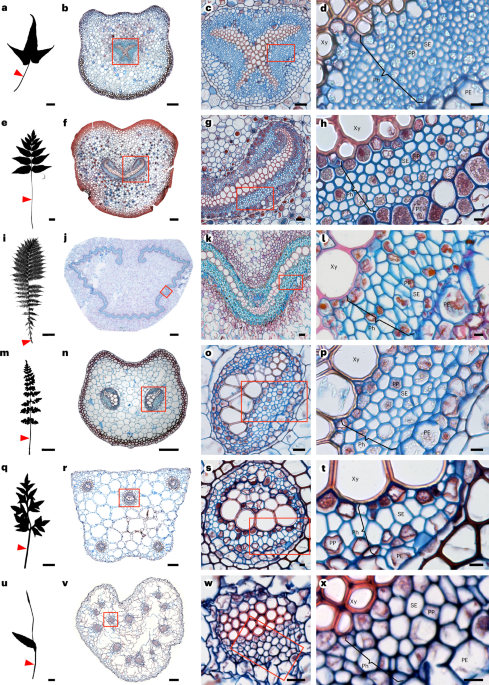
To quantify the SE radius, individual SEs were first outlined manually with the ‘Freehand selections’ tool, and the selected regions were used to create a mask for area measurements. Areas of the masks were quantified with the ‘Analyze Particles’ (ImageJ) function. The radius was then calculated with \({\rm{radius}}=\sqrt{\frac{\rm{area}}{\pi }}\). The SEs were counted for one sample per species in ImageJ. For single-vascular-bundle species (for example, Asplenium hemionitis and Anemia mexicana; Fig. 1b,f), all SEs were counted. For double-vascular-bundle species (for example, Cystopteris fragilis; Fig. 1n), SEs in one side of phloem were counted and the number was multiplied by two to yield an estimation of total SE number. In Thelypteris palustris and Osmunda regalis, the SE numbers were very large, and the SEs exhibited a repeating pattern throughout the vasculature (Fig. 1j,k). Therefore, all SEs within a certain phloem area (for example, Fig. 1k) were counted and used to estimate the total SE number based on the proportion of this phloem area relative to the total phloem area. For the asymmetric vascular bundles in Pteridium aquilinum, all SEs were counted manually. For the very large species Aangiopteris evecta, all SEs in one eighth of the petiole were counted, and we calculated the total SE number by multiplying the number by eight.

Quadrat sampling of SEs for extant ferns

Five sampling squares were placed across the phloem area to capture more than 50 SEs on each image. The placement of sampling squares on each sample was based on the types of vascular architecture, categorized according to the number of vascular bundles. These types include single-bundle (Fig. 1b,f,j and Extended Data Fig. 4a), double-bundle (Fig. 1n and Extended Data Fig. 4b) and multiple-bundle (Fig. 1r,v and Extended Data Fig. 4c) bundle types. The multiple-bundle type was then subgrouped into symmetric (Fig. 1r and Extended Data Fig 4c) and asymmetric arrangements. For the single-bundle type, five sampling squares were placed across the phloem randomly. For the double-bundle type, because the two vascular bundles were symmetrical, five sampling squares were placed randomly across the phloem on one of the vascular bundles. For the symmetric multiple-bundle type, five sampling squares were placed on each vascular bundle. In all cases, when the number of SEs in each vascular bundle was less than ~50, quadrat sampling was not applied and all SEs were measured instead. For the asymmetric multiple-bundle type (Pteridium aquilinum), all SEs were measured because vascular bundles of various sizes were distributed randomly in the petiole. In this case, more than 4,000 SEs had to be manually masked, so the number of individuals was reduced to one for this species. The vasculature architecture in Angiopteris evecta also belongs to the asymmetric multiple-bundle type, but because of the extremely large number of SEs (~10,000), all the SEs in a one-eighth section of the petiole were measured. This included 1,252 measurement of the SE radius.

To ensure the consistency of our strategy, we compared the datasets generated with our sampling strategy to complete datasets with all SEs measured. This was carried out for five spices representing the single (Salvinia auriculata, Adiantum aleuticum), double (Asplenium viride, Onoclea sensibilis) and symmetric multiple (Platycerium bifurcatum) types (Extended Data Fig. 4). The comparison between sampled datasets and full datasets showed no significant differences (Kruskal–Wallis rank sum tests, P > 0.05; Extended Data Fig. 2 and Supplementary Table 12); therefore, the sampling strategy was applied to these vascular types.

Testing and quantifying intraspecific and interspecific differences

Due to the non-normal distribution of SE radius data confirmed by Shapiro–Wilk tests and visual inspection of histograms, non-parametric methods were used to evaluate differences among groups. The median value of the SE radius in each sample was used to represent the individual SE radius, and the mean value of the individual SE radius of the same species was used to represent the species SE radius. A Kruskal–Wallis (KW) rank-sum test was performed to assess overall between-species differences. All statistical analyses were conducted in R using the kruskal.test() function from the stats package. The effect sizes ηH2 of the KW test were calculated with the kruskal_effsize() function in the ‘rstatix’ package (version 0.7.3)55. Intraspecific and interspecific variation were also quantified using the s.d. and c.v., also calculated in R. Because many species were represented by only three individuals, and some by only a single individual, Dunn’s test had limited power for pairwise post hoc comparisons. Therefore, to confirm that significant interspecific differences were not caused by extreme values, we performed KW tests with a dataset excluding the species with the largest values, Angiopteris evecta, and a dataset excluding both A. evecta and the species with the second largest values, Osmunda regalis (Supplementary Table 4). The s.d. and c.v. were calculated accordingly (Supplementary Table 5).

Investigating scaling relationships with PGLS

We estimated the scaling relationships between SE radius and leaf morphological or vascular anatomical traits using PGLS models. The five traits—leaf area, leaf length, vascular bundle radius, vascular sectoriality index and circularity—were treated as predictor variables, and SE radius was treated as the response variable. Species means were calculated from individual median values and used to represent each species in the models. SE radius, leaf area, leaf length, vascular bundle radius and sectoriality index data were log10-transformed before being fitted into the models to increase normality (Extended Data Fig. 5). Among the 26 sampled species, 23 species had data for all five traits and 2 species had only vascular traits. First, 25 species were included in the models with vascular traits as predictor variables (model names: PGLS_V, PGLS_Sec, PGLS_Cir), and 23 species were included in the models with leaf traits as predictor variables (model names: PGLS_LA, PGLS_LL). For comparisons among the five predictors and to identify the best predictors, the dataset of 23 species was also fitted into the models with vascular traits as predictor variables (model names: PGLS_V_n23, PGLS_Sec_n23, PGLS_Cir_n23). In the models PGLS_V_Lep, PGLS_Sec_Lep and PGLS_Cir_Lep, only data from leptosporangiates were used. To explore whether adding predictors to a model would increase model fit, we developed models with two predictors under all possible combinations using the dataset of 23 species without missing data (Supplementary Table 7). Principal component analysis was used to examine the collinearity of the five predictor variables (Extended Data Fig. 6).

Comparisons between models were based on AIC, and a ΔAIC of 2 was considered significant. A model with a lower AIC value is better supported. Phylogenetic trees matched to the dataset were extracted from the Fern Tree of Life (FTOL) with the R package ‘ftolr’ (version 1.6.0)19,56. We used Pagel’s λ (ref. 32) to estimate phylogenetic signals within PGLS models. We performed the analyses in R with ‘phylolm’ (version 2.6.5)57. Quantile–quantile and residuals versus fitted values plots were used for assessing assumptions in the PGLS models (Extended Data Fig. 5).

ASR and phylogenetic signals

A phylogenetic tree of sampled species was extracted from the FTOL with the R package ‘ftolr’ (version 1.6.0)19,56. We performed ASR and calculated phylogenetic signals with the R package phytools58. ASR was based on maximum likelihood and carried out using the fastAnc() function, which uses maximum likelihood under a Brownian motion assumption. The result was visualized with the contMap(), colorRampPalette() and setMap() functions in phytools. The phylogenetic signal of the SE radius was quantified by both Blomberg et al.’s K (ref. 31) and Pagel’s λ (ref. 32) using the phylosig() function.

Anatomical data collection for fossilized phloem and comparisons between the measurements of extant and extinct species

We combined a literature survey with an investigation of thin fossil sections in museum collections. Based on our literature survey, fossilized phloem has been well characterized in several extinct fern species (summarized in Supplementary Tables 8 and 13). These species include Sphenophyllum plurijoliatum (Equisetales)34, Psaronius sp. (Marattiales)36, Botryopteris tridentata (leptosporangiates)37, Anachoropteris involuta (leptosporangiates)38 and the early fernlike plants Etapteris leclercqii (Zygopteridales)37 and Stauropteris biseriata (Stauropteridales)59. For these species, SEs were measured directly based on published images with either scale bars or magnification factors using ImageJ. We also rephotographed two specimens of Sphallopteris schlechtendali in the Hunterian Museum, the University of Glasgow (Supplementary Table 8). In addition, we imaged samples of Stauropteris burntislandica (Fig. 5a–c) in the Cockburn Geological Museum, the University of Edinburgh.

We identified SEs in fossils according to the published literature, as summarized in Supplementary Table 13. In published studies, phloem and SEs were characterized using both transverse and longitudinal sections, allowing SEs to be identified as elongated cells, with tapered end walls and sieve areas and pores. In summary, there were three scenarios for different species:

(1)

In E. leclercqii, B. tridentata and A. involuta, there are no parenchyma cells between SEs, so the measurements were taken entirely on SEs.

(2)

In Psaronius sp. and S. burntislandica (according to the reference of Stauropteris biseriate59), both SEs and phloem parenchyma cells can be observed in phloem, but they are not distinguishable from each other in transverse sections where measurements should be taken. Therefore, we measured all phloem cells.

(3)

In Sphenophyllum pluriioliatum, Tempskya dernbachii (primary phloem) and S. schlechtendali, it is unknown whether the phloem contains parenchyma cells, so all phloem cells were measured.

To ensure that the possible inclusion of parenchyma cells in fossil samples did not affect our conclusions, we measured them in the extant members of Equisetales, Osmundales and Marattiales and compared the data to their SEs as well as the phloem cells in their extinct relatives (Extended Data Fig. 7). The radii of both cell types measured in extant species are larger than those of phloem cells in their extinct relatives, supporting the robustness of our inference that phloem conducting cells show a decreasing trend in radius through time.

All the measurement taken from samples prepared with the cellulose acetate peel technique were corrected by a ×1.05 factor due to shrinkage caused by the peeling technique60. In Psaronius sp., S. pluriioliatum, T. dernbachii, S. schlechtendali and S. burntislandica, both SEs and phloem parenchyma cells were present but were not distinguishable with each other in cross-section images according to the literature. Therefore, all phloem cells were measured and used for analysis. Significance tests between fossils and extant ferns were done with KW tests, as described above.

Finally, we ensured the robustness of our comparisons between extant ferns and fossils by carefully accounting for the nature of both datasets. In living species, we chose the MPOP as our standard sampling location as we identified it as the position with the largest SE radius. However, in fossils, we had no control over the sampling location along the petiole, so we assumed that many were not from the largest SEs at the MPOP. The observation that extinct SE radii were still larger in fossils adds weight to the conclusions that SE radius has decreased through time. Additionally, we wanted to ensure that our results were not biased by the presence of a type of distinctively large SEs present only in the extinct species A. involuta38 and Psaronius sp.36 and also observed in S. burntislandica in this study (Fig. 5c). This small number of large SEs are distinctively wider than the majority of SEs38. However, removing these very large SEs did not change the conclusions that SE radii in fossils are significantly larger than those in extant plants (Supplementary Table 10). With the consideration of these potential caveats, our results provide strong evidence for a decrease in SE radius through time.

Mathematical modelling of phloem conductivity

SEs are approximately circular cylindrical vessels with radius a, which, in all the extant ferns, lie in the range from a ≈ 1.9 μm to a ≈ 13.5 μm (Fig. 2). The flow is driven by an osmotic pressure difference Δp generated by the loading of sugars in the source tissue and the unloading of photo-assimilates in the sinks. The speed v at which carbohydrates travel can be estimated from the mechanics of incompressible Newtonian fluids, which are governed by Navier–Stokes equations (or Newton’s second law). The average speed is

$$v=\frac{{a}^{2}}{8}\frac{\Delta p}{\eta L},$$

where L is the source-to-sink distance and η ≈ 2 mPa s is the sap viscosity based on an ~20% wt solution61. This equation, sometimes called Darcy’s law, is valid under low-Reynolds-number conditions, where viscous friction dominates the flow. The total flow rate Q = Av can be found by multiplying the conductive area A by the speed v.

An important feature of Darcy’s law is that the speed scales with the radius squared: doubling the radius leads to a fourfold increase in the sugar-transport capacity. To illustrate this, we assume a translocation distance of L = 1 m and a pressure drop of Δp = 0.1 MPa. This leads to speeds that vary ~50 times (v ≈ 0.021 to 1.14 mm s−1), although the radius increases only by less than a single factor of ten (a ≈ 1.9 to 13.5 μm). This prediction is not inconsistent with the experimental data; see, for example, ref. 5.

In summary, we note that all information about the phloem SE geometry is contained in the factor a2/8, which we identify as the permeability: k = a2/8. Its magnitude, k = 0.45 to 22.78 μm2 (a ≈ 1.9 to 13.5 μm), allows us to gauge the relative performance of different species.

Finally, we note that it is possible to include additional effects in the analysis: for example, variations in sugar concentration, flow across sieve plates or potential wall slip, but we did not do that here.

Statistics and reproducibility

The microscopic images of extant species presented in Fig. 1 and Extended Data Figs. 1 and 2 are representative anatomical observations of phloem tissue. The anatomical features shown were consistently observed across all the samples examined for each species, with individual numbers summarized in Supplementary Table 1. The microscopic images in Fig. 5a–c come from a single fossil specimen containing seven petiole cross-sections of S. burntislandica. The largest and best-preserved section, shown in Fig. 5a–c, was selected as representative.

Reporting summary

Further information on research design is available in the Nature Portfolio Reporting Summary linked to this article.