
Experimental details
The experimental results presented in this paper were obtained using the Gemini laser system. A DPM system is used to improve the laser contrast to Imax/I(t) > 108 at times more than 1 ps before the peak of the pulse, whereas the sub-ps contrast is discussed in the text referring to Fig. 1. A total throughput of 50% was measured, which leads to on-target pulse energies of 5 J in the 50 ± 5 fs duration pulses with λL = 800 nm, which are focused by an f/2 parabola onto a polished fused silica target.
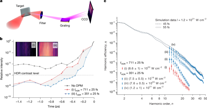
Pulses with energies of up to 12 J (before DPM system) in 50 ± 5 fs at a central wavelength of 800 nm were used, which, when focused to a FWHM spot size of 2 μm, reach peak intensities I > 1021 W cm−2. As shown in Fig. 1a, these were focused onto optical-grade fused silica targets in p-polarization at an incidence angle of 45°, and the spectrum of extreme ultraviolet radiation emitted in the direction of specular reflection was recorded.
The on-target intensity was varied by apodizing the beam, which both reduces the laser pulse energy and increases the focal spot size but maintains the same near-field intensity so that the DPM response and contrast are unchanged. The reflected harmonic beam was detected using a cylindrically curved XUV flat-field spectrometer consisting of a 300 lines per mm grating imaging the source in the spectral dimension. Aluminium filters with thicknesses ranging from 0.2 μm to 3 μm were used to attenuate optical emission. No focusing optic was used so that the XUV signal is incident directly onto the charge-coupled device (CCD). The harmonic spectra were detected using a back-thinned ANDOR CCD (Andor DV436) with a resolution-limited pixel size of 13.5 μm placed 1.2 m from the interaction point.
The plasma density gradient was controlled by a 25 mm diameter, 3 mm thick fused silica substrate with an anti-reflection coating on the front side and high reflectivity on the rear. This pick-off mirror was inserted into the main beam line in front of the last mirror before the parabola. This introduced a prepulse, which is focused by the same parabola as the main beam onto the target but with a lower intensity because of the larger focal spot size. Precise adjustment of the distance between the substrate and the full-beam mirror allowed for prepulse timing to be controlled to within 25 fs of the main pulse. This fine timing control enabled accurate tailoring of plasma expansion before the arrival of the driving pulse.
Laser contrast enhancement was achieved through measurements that determined that the anti-reflection coating on the first plasma mirror (PM) of the DPM was breaking down too early in the rise time of the native (unaltered) Gemini pulse contrast. This resulted in the ‘slow rise time’ DPM configuration (tHDR = 711 ± 25 fs; Fig. 1b, red trace). By replacing the first PM with an uncoated substrate, we improved the DPM performance to have a tHDR = 351 ± 25 fs (Fig. 1b, blue trace). The motivation for making this change comes from a separate branch of study on ultrafast materials science that focuses on the part played by materials that are highly structured on the nanoscale in the lifetime of excited electrons before material breakdown45,46. Note that for different peak intensities, tHDR will describe different absolute intensities, whereas the ratio remains the same. This should, therefore, be considered carefully in the context of a given peak intensity interaction.
Harmonic energy deconvolution
To obtain the overall efficiency, the spectral response as a function of wavelength, λ, of all components of the spectrometer were accounted for separately as indicated by
$$S(\lambda )=\text{Al}\times \text{QE}\times \text{G}\,\times {\text{Al}}_{2}{\text{O}}_{3}\times \text{CH},$$
(1)
where Al is the aluminium filter transmission47 (0.2–3 μm), QE is the quantum efficiency of the back-thinned Andor DV436 (ref. 48), G is the calculated efficiency of the SHIMADZU-L0300-20-80 flat-field grating49, Al2O3 is the contaminant aluminium oxide layer present on the filters (see aluminium oxide layer calibration below) and CH is the hydrocarbon contaminant layers47.
The energy per count is calculated as
$$E(\lambda )=\frac{G\times S(\lambda )\times \varepsilon \times {q}_{{\rm{e}}}}{{\rho }_{{\rm{f}}{\rm{r}}{\rm{a}}{\rm{c}}}}$$
(2)
where G = 2 is the number of electrons per count (e− per count), ε is the average energy required to produce an electron–hole pair in silicon, 3.65 eV, qe is the electronic charge and ρfrac is the fraction of the beam incident onto the CCD. This is restricted by the angle of acceptance of the flat field grating of 3.66 mm and the camera chip width of 27.6 mm. We assume a two-dimensional (2D) Gaussian beam propagating along the z-axis, with its transverse intensity profile described by
$$G(x,y)=\exp \left(-\left[\frac{{(x-{x}_{0})}^{2}}{2{\sigma }_{x}^{2}}+\frac{{(y-{y}_{0})}^{2}}{2{\sigma }_{y}^{2}}\right]\right),$$
(3)
where (x0, y0) is the centre of the beam and σx and σy are the standard deviations of the beam along the x- and y-directions, respectively (measured values of beam divergence are used). We need to compute the fraction of the total beam that falls within a rectangular aperture defined by
$$x\in [{x}_{\min },{x}_{\max }],y\in [{y}_{\min },{y}_{\max }].$$
This fraction is given by the ratio
$${\rho }_{\text{frac}}=\frac{{\int }_{{y}_{\min }}^{{y}_{\max }}{\int }_{{x}_{\min }}^{{x}_{\max }}G(x,y){\rm{d}}x{\rm{d}}y}{{\int }_{-\infty }^{\infty }{\int }_{-\infty }^{\infty }G(x,y){\rm{d}}x{\rm{d}}y}$$
(4)
The total Gaussian beam over all space is \(2{\rm{\pi }}{\sigma }_{x}{\sigma }_{y}\) thus,
$${\rho }_{{\rm{f}}{\rm{r}}{\rm{a}}{\rm{c}}}=\frac{1}{4}\,\left[{\rm{e}}{\rm{r}}{\rm{f}}\,(\frac{{x}_{max}-{x}_{0}}{\sqrt{2}{\sigma }_{x}})-{\rm{e}}{\rm{r}}{\rm{f}}\,(\frac{{x}_{min}-{x}_{0}}{\sqrt{2}{\sigma }_{x}})\right]\times \left[{\rm{e}}{\rm{r}}{\rm{f}}\,(\frac{{y}_{max}-{y}_{0}}{\sqrt{2}{\sigma }_{y}})-{\rm{e}}{\rm{r}}{\rm{f}}\,(\frac{{y}_{min}-{y}_{0}}{\sqrt{2}{\sigma }_{y}})\right]$$
(5)
By measuring the beam divergence (Fig. 3), we then calculate the associated fraction ρfrac of the beam that was incident onto the CCD. The uncertainty in the energy deconvolution is dominated by systematic uncertainty in the thickness of surface oxide (Al2O3), carbon contamination layers (CH) and the beam divergence measurement (ρfrac). The correction is estimated by evaluating it at two extreme limits and then taking half the difference between the resulting corrected values as a symmetric uncertainty bound.
Aluminium oxide layer calibration
A 2.15 μm thick aluminium foil, which was used as a filter for the harmonic signal, was imaged at the Ewald Microscopy Centre, Queen’s University Belfast, to determine the thickness of the oxide containment layers. A cross-sectional lamellae was prepared using a Tescan focused ion beam scanning electron microscope (SEM) Lyra3, which can be seen in Extended Data Fig. 3a. High-angle annular dark-field imaging was performed, which images the front surface of the aluminium foil. Moreover, energy-dispersive X-ray (EDX) mappings were performed on this section of the lamellae, exhibiting a difference in the layer structure. Elemental mapping was used across the foil to identify the oxygen region corresponding to the aluminium oxide formed on the surface. The thickness of the oxide layers was observed to vary between 7 nm and 16 nm as seen in Extended Data Fig. 4b. This is consistent with the native oxide typically formed on aluminium exposed to ambient conditions. However, it differs from other studies that measured the oxide layer thickness as 8 nm in total, not just the front surface thickness as measured here50. This variation of oxide layers has been included in the experimental uncertainties in the presented energy calculations. The need for gold sputtering of the sample surface and the low signal yield from light elements make it difficult to measure the hydrocarbon contaminant layer on the sample; we refer to ref. 50 for this value.
Grating second and third orders
Using a diffraction grating to image XUV harmonics, the appearance of features at what seem to be ‘half-order’ or ‘third-order’ harmonic positions is attributed to the higher diffraction orders of the grating appearing with the first-order signal. In Extended Data Fig. 5a, the lower-order harmonic region of the XUV spectrum between 47 nm and 45 nm, there are apparent ‘half-order’ harmonics observed. However, when comparing these features to the higher-order harmonics shown in Extended Data Fig. 5b between 20 nm and 22.5 nm, it can be seen in the magnified region of the plots that the half harmonic order that is seen to be at 19.5th order is actually the 39th-order harmonic being imaged in second order because of the matching spatial and spectral shape of these two images.
This highlights the importance of accounting for second- and even third-order diffraction contributions when analysing and calculating the total energy distribution in the lower-order spectral region. Using an aluminium filter allows transmission of certain XUV wavelength ranges while blocking others. By choosing a filter that transmits only the desired harmonic range and blocks shorter wavelengths, we can suppress unwanted second- or third-order contributions. However, using a 300 l mm−1 grating in the wavelength range of 80–20 nm, signals close to the aluminium L-edge cut-off can appear in the second and third order with the lower-order harmonics.
In Extended Data Fig. 6a, the ratio of the first and second diffraction orders of the measured SHIMADZU-LO300 flat-field grating is shown49. This was measured using the laser-driven high harmonics that were incident onto a pinhole. It is seen in Extended Data Fig. 6a that the second-order efficiency approaches the first-order efficiency at higher frequencies. In Extended Data Fig. 6b, the ratio of the first and third diffraction orders are shown, which has a similar trend in approaching the first order when moving towards higher frequencies.
A logistic function was fitted to the data
$${R}_{\frac{{S}_{2,3}}{{S}_{1}}}(n)=\frac{v}{1+{{\rm{e}}}^{-k(n-{n}_{0})}}+b,$$
(6)
where, for the second diffraction order, v = 0.92, n0 = 40, k = 0.37 and b = 0.12 and for the third diffraction order, v = 0.79, n0 = 44, k = 0.44 and b = 0.13. Failing to account for these effects leads to overestimating the reflected harmonic energy in the lower orders, for which the aluminium filter attenuates the spectrum considerably. The trend given by equation (6) was used to account for the second- and third-order diffraction contributions. Owing to this overlap being unavoidable, using the grating response, we can deconvolve the overlapping orders from the spectrum.
Numerical simulations
The SHHG interaction was modelled using high-resolution 2D simulations performed with the PIC code Smilei51. A spatial resolution of 512 cells per laser pulse wavelength and a temporal resolution of 1,024 timesteps per laser pulse cycle were used, enabling the resolution of harmonics beyond the aluminium L-edge (17 nm) (ref. 28). The p-polarized laser pulse is incident on a fully ionized SiO2 target of number density 6.62 × 1023 cm−3 with an exponential preplasma ramp. Optimal preplasma scale lengths for XUV SHHG efficiencies were determined from one-dimensional (1D) PIC simulations and ranged from 0.12λL to 0.16λL. XUV SHHG efficiencies are typically optimized for scale lengths in the range of 0.1–0.2λL (refs. 23,37,52). Particles are initialized with 100 macro-electrons per cell at a temperature of 115 eV and 4 macro-ions per species per cell at zero temperature. The laser pulse is modelled as a spatiotemporal Gaussian with a spatial FWHM of 2 μm and a temporal FWHM of 45 fs and 55 fs. As the pulse duration is anticipated to influence the attainable absolute efficiencies in the specularly reflected harmonic cone, simulations were performed to bound the range sampled in the experiment due to shot-to-shot variations (±5 fs), therefore yielding a range of optimized efficiency values (Fig. 1c, grey shaded area). Silver Müller boundary conditions allow the free movement of particles and electromagnetic fields into and out of the simulation window53. Smilei’s in-built Bouchard solver54 is applied to reduce the error from numerical dispersion in 2D inherent to traditional finite difference solvers55. It has been shown that modifications to the finite difference approach can sufficiently reduce this error56.
Normalized vector potential
It is standard practice in PIC simulations to define the normalized vector potential, a0, instead of intensity. For a laser pulse of frequency, ω, and peak electric field amplitude, E, corresponding to an intensity, \(I=\frac{1}{2}c{{\epsilon }}_{0}{E}^{2}\), the normalized vector potential is expressed as \({a}_{0}=\frac{{eE}}{{m}_{{\rm{e}}}c\omega }\), where c is the speed of light, ϵ0 the vacuum permittivity and me the mass of an electron. In particular, the onset of relativistic effects, including SHHG, occurs for a0 ≥ 1. In Fig. 1c, an a0 of 24 is used in the PIC simulation to model the interaction. In Fig. 2, a0 values ranging from 2 to 25 are used to explore the parameter space and in Fig. 2b,c, the a0 values are 13 and 21, respectively. An a0 of 25 is used in Fig. 4b.
Analytical model of XUV beam profiles
In reality, the plasma surface is not expected to remain flat over the entire duration of the Gemini laser pulse. The steep intensity gradients result in a ponderomotive force, initially deforming the plasma surface into a concave ‘dent’ that follows the profile of the central maximum of the focal spot. The dent depth Δz, defined as the difference between the position of the critical density surface at the spatiotemporal peak of the driving laser pulse and its original position, is calculated from an analytical model22 detailed below for the experimental conditions and compared with 2D PIC simulations with the same parameters. An intensity-dependent phase term is included in the far-field harmonic beam profile model to account for this denting.
The Fraunhofer diffraction equation describes the propagation of a monochromatic, λ, scalar field amplitude to large distances as a Fourier transform. It describes the propagation of a focused laser pulse from its far-field profile, U0(x′, y′), to its near-field profile, U(x, y, z), as
$$U(x,y,z) \sim \iint {U}_{0}({x}^{{\prime} },{y}^{{\prime} }){{\rm{e}}}^{-2\mathrm{\pi i}({f}_{x}{x}^{{\prime} }+{f}_{y}{y}^{{\prime} })}\text{d}{x}^{{\prime} }\text{d}{y}^{{\prime} } \sim {\mathcal{F}}({U}_{0}({x}^{{\prime} },{y}^{{\prime} })){|}_{{f}_{x}=x/\lambda z,{f}_{y}=y/\lambda z},$$
(7)
where z is the distance from the focal spot. The far-field nth harmonic spatial profile is modelled by applying the theory of relativistic spikes10. Writing this adjustment as \(S=S(n,{a}_{0}({x}^{{\prime} },{y}^{{\prime} }))\), which contains a sharp roll-off at a harmonic order that scales as \({a}_{0}^{3}\), the far-field amplitude of the nth harmonic is
$${U}_{0}({x}^{{\prime} },{y}^{{\prime} },n) \sim \sqrt{S(n,{a}_{0}({x}^{{\prime} },{y}^{{\prime} }))}{U}_{0}({x}^{{\prime} },{y}^{{\prime} }).$$
(8)
Propagating the far-field harmonic beam profile to the near-field,
$$U(x,y,z,n) \sim {\mathcal{F}}({U}_{0}({x}^{{\prime} },{y}^{{\prime} },n)){|}_{{f}_{x}=x/{\lambda }_{n}z,{f}_{y}=y/{\lambda }_{n}z}$$
(9)
where λn is the wavelength of the nth harmonic.
Radiation pressure of the laser pulse on the target surface causes a curvature of that surface, Δz = Δzi + Δze, composed of the motion of the ion profile, Δzi, and the excursion of the electrons, Δze. This curvature is modelled with the addition of a phase term, \({\phi }_{n}=2{k}_{n}\Delta z\cos \theta \), to the far-field profile. A previous study provided a model for Δz (ref. 22). For the Gemini pulse duration, the surface curvature varies slowly in time around the peak of the laser pulse, at tp, when most harmonic emission occurs. The ion surface dent produced by a laser pulse with normalized vector potential aL(x′, y′, t′) incident at an angle θ on an exponential preplasma of scale length L is
$$\Delta {z}_{\text{i}}({x}^{{\prime} },{y}^{{\prime} })=2L\mathrm{ln}\,\left(1+\frac{{\varPi }_{0}}{2L\cos \theta }{\int }_{-\infty }^{{t}_{\text{p}}}{a}_{\text{L}}({x}^{{\prime} },{y}^{{\prime} },{t}^{{\prime} })\text{d}{t}^{{\prime} }\right)$$
(10)
where \({\varPi }_{0}={({RZ}{m}_{\text{e}}\cos \theta /2A{M}_{\text{p}})}^{1/2}\); R is the reflectivity of the relativistic plasma mirror; Z and A are, respectively, the average charge state and mass number of the ions; me is the electron mass and Mp is the proton mass. The electron excursion is
$$\Delta {z}_{\text{e}}({x}^{{\prime} },{y}^{{\prime} })=2L\mathrm{ln}\,\left(1+\frac{2{a}_{\text{L}}({x}^{{\prime} },{y}^{{\prime} })(1+\sin \theta )}{2{\rm{\pi }}{(\cos \theta )}^{2}L/\lambda }{{\rm{e}}}^{-\Delta {z}_{\text{i}}/L}\right).$$
(11)
Extended Data Fig. 7 compares the analytically calculated dent from ion motion to 2D PIC simulations with laser pulse intensities consistent with the shots of Fig. 3. Reflectivities are extracted from the simulations. Accounting for the corresponding phase term, the near-field intensity profile of the nth harmonic is
$$I(x,y,z,n) \sim {|{\mathcal{F}}(\sqrt{S(n,{a}_{0}({x}^{{\prime} },{y}^{{\prime} }))}{U}_{0}({x}^{{\prime} },{y}^{{\prime} }){{\rm{e}}}^{-2{\rm{i}}{k}_{n}\Delta z({x}^{{\prime} },{y}^{{\prime} })\cos \theta }){|}_{{f}_{x}=x/{\lambda }_{n}z,{f}_{y}=y/{\lambda }_{n}z}|}^{2}.$$
(12)
We note that additional contributions to harmonic focusing may arise from intensity-dependent shifts of the apparent reflection point predicted by relativistic similarity theory57,58. Overall, this modelling demonstrates that, as well as increased energy in the harmonic beam, the experimental demonstration of the theoretically efficiency-optimized regime is also confirmed by (1) an intensity-dependent reduction in spatial filtering (departure from Gaussian-like beam profile); (2) a rapid, intensity-dependent growth in divergence; and (3) strong spectrospatial modulations in the emitted harmonic beam. The second and third points are also indications of efficient emission from a concave-dented plasma.
Although a CHF was not measured directly in this work, the observation of rapid increases in beam divergence with intensity, accompanied by the emergence of strong spectrospatial modulations provides evidence for the generation of CHF-suitable conditions in this experiment. This is further supported by 2D simulations, which predict the formation of a CHF during the experiment (Fig. 4). In the future, some degree of independent control of the plasma surface curvature is necessary to optimize both SHHG and the CHF performance simultaneously. This control could be passive, that is, a pre-shaped target that compensates for induced curvature, or active—that is, use of a substantially longer prepulse in conjunction with a single or few-cycle high-power driving laser pulse to exert absolute control over the shape of the surface at the moment of generation.
It remains uncertain how the spectrospatial modulations observed in this work will interplay with the spatiotemporal couplings that become increasingly more impactful at multi-PW levels, but techniques are now available for on-shot quantification of these couplings59. Moreover, although spatiotemporal laser–plasma couplings can play a substantial part in the quality of a CHF, in the efficiency limit, simulations show that these are dominated, and so can be controlled, by the driving field of the incident laser pulse3,60.
CHF 3D gain convergence
The CHF gain in 3D was estimated using 2D PIC simulations, following the methodology in ref. 39. The electromagnetic field intensities of the reflected harmonic beam are extracted from 2D PIC simulations at the time of generation of the brightest CHF, If, and at the time of generation of the attosecond pulse that produces this CHF, I0. The snapshot of Fig. 4b is taken at the time of generation of the brightest CHF. The 3D boost can now be calculated. First, the gain from temporal compression, ΓD, is I0/IL, where IL is the intensity of the incident laser pulse. The 2D gain from spatial compression is Γ2D = If/I0. The 3D gain that can be anticipated from spatial compression is \({\varGamma }_{3\text{D}}={\varGamma }_{2\text{D}}^{2}\) and the full 3D gain is Γ = ΓDΓ3D. The attosecond pulses of Fig. 4a are then scaled using these equations and making the approximation that temporal gain is constant. As high harmonic orders contribute substantially to the intensity at the CHF, the accurate measurement of gain requires an unfeasible simulation resolution. To test the quality of the resolution used for the analysis, a scan of gain as a function of simulation resolution is plotted in Extended Data Fig. 8. A lower bound on the gain of 88 is extracted from the highest accessible resolution simulation, but higher gains seem probable.