
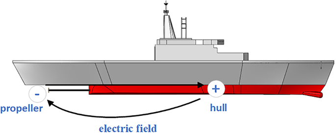
Current sources or electric dipoles are the basic units for the inversion of underwater electromagnetic fields of targets such as vessels. Previous studies have shown that due to the differences in electrical conductivity between the air layer and seabed layer in the marine environment relative to seawater, the distribution of underwater electric fields in the marine environment is significantly affected by different media. As a special medium, sea ice also often has a non-negligible impact on the distribution of underwater electric fields in polar and other low-temperature sea areas40. Therefore, this paper takes the current source in the four-layer medium of sea-ice-covered areas (such as polar regions) as the basic research unit, as illustrated in Fig. 2, and focuses on analyzing the distribution of its underwater electrostatic field under the influence of the ice layer. Consider a horizontally stratified four-layer medium representing the polar marine environment. The domain is defined within a Cartesian coordinate system \((x,y,z)\) where the z-axis denotes depth. The individual layers are characterized by their respective macroscopic electrical conductivities \({\gamma _n}\) (\(n \in \{ 1,2,3,4\}\)), which represent the air (\({\gamma _1}\)), sea ice (\({\gamma _2}\)), seawater (\({\gamma _3}\)), and seabed (\({\gamma _4}\)). The parallel planar interfaces between these domains are located at depths \(z = {z_1}\) (air-sea ice, namely BC1), \(z = {z_2}\) (sea ice-seawater, namely BC2), and \(z = {z_3}\) (seawater-seabed, namely BC3). A horizontal current source pair, constituting a generalized dipole with positive current \(+ I\) and negative current \(- I\) separated by a discrete distance 2a, is submerged strictly within the high-conductivity seawater layer (Layer 3) at an operational depth \({z_0}\). However, it should be noted that in actual marine environments, sea ice is a complex composite consisting of pure ice, brine pockets, and air bubbles. Due to the intricate internal pore structures and the heterogeneous distribution of brine pockets among ice crystals, the electrical conductivity of the ice layer is non-uniformly distributed, with localized regions of higher conductivity. Such complexity is difficult to faithfully simulate under engineering and laboratory conditions. Therefore, this paper proposes a simplified four-layer medium model, in which the electrical conductivity of each layer is assumed to be homogeneous.
Fig. 2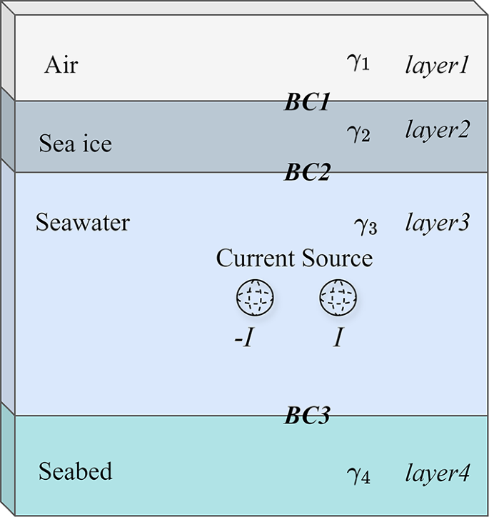 General formulation of the multilayer boundary value problem
Current sources or electric dipoles serve as the fundamental analytical units for the inversion of underwater electromagnetic fields generated by submerged targets such as vessels. While previous analytical frameworks, notably the foundational four-layer horizontal electric dipole model rigorously established by Wołoszyn, have successfully addressed the “air-seawater-seabed-non-conductive layer” stratification prevalent in shallow coastal waters34, the presence of polar sea ice introduces structurally distinct electromagnetic boundary conditions. Therefore, this paper constructs an adapted four-layer analytical model specifically tailored for polar regions, wherein the sea ice acts as an intermediate finite-thickness layer exerting profound conductive constraints.
In the steady-state static regime, the spatial electric field E is irrotational, which means it satisfies:
$$E = – \nabla \varphi $$
(1)
By combining the microscopic form of Ohm’s law (\(J = \gamma E\)) with the continuity equation for steady currents (\(\nabla \cdot J = \nabla \cdot {J_{source}}\)), the scalar electrical potential \( {\varphi _n} \) within each homogeneous layer must satisfy either the Poisson equation (within the source layer) or the Laplace equation (within source-free regions):
$${\nabla ^2}{\varphi _n} = – \frac{1}{{{\gamma _n}}}\nabla \cdot {J_{source}}{\delta _{n,3}}$$
(2)
where \( {\delta _{n,3}}\) is the Kronecker delta function indicating that the physical source resides exclusively in Layer 3.
The absolute uniqueness of the potential distribution throughout the entire multi-layered domain is strictly governed by the Dirichlet and Neumann boundary conditions enforced at each geometric interface \(z = {z_k}\):
(1)
Continuity of the scalar potential \({\varphi _k}(x,y,{z_k}) = {\varphi _{k + 1}}(x,y,{z_k})\) \(\forall (x,y) \in \mathbb{R}^{2},k \in \{ 2,3\}\);
(2)
Continuity of the normal component of the current density \({\left. {{\gamma _k}\frac{{\partial {\varphi _k}}}{{\partial z}}} \right|_{z = {z_k}}} = {\left. {{\gamma _{k + 1}}\frac{{\partial {\varphi _{k + 1}}}}{{\partial z}}} \right|_{z = {z_k}}} \) \(\forall (x,y) \in \mathbb{R}^{2},k \in \{ 2,3\} \).
Furthermore, at the uppermost boundary delineating the interface between the air and the sea ice surface (\(z = {z_1}\)), the practically infinite resistance of the air layer (\({\gamma _1} \approx 0\)) mathematically enforces a zero-flux Neumann boundary condition:\({\left. {\frac{{\partial {\varphi _2}}}{{\partial z}}} \right|_{z = {z_1}}} = 0\), ensuring no current escapes into the atmosphere.
Analytical solution via the successive reflection series expansion
To resolve the coupled boundary value problem without resorting to computationally intensive volumetric numerical discretization (e.g. FEM), we employ the method of successive reflection series expansions. While conventional approaches often visualize this through discrete heuristic image geometries, the problem is fundamentally an algebraic boundary matching sequence.
When a primary electrostatic potential field, originating in a host medium with conductivity \({\gamma _i}\), propagates and impinges upon an impedance boundary with an adjacent medium of conductivity \({\gamma _j}\), it inevitably generates a reflected potential field back into the host medium. The relative magnitude of this boundary reflection is rigorously quantified by the electrostatic reflection coefficient \({\Gamma _{i,j}}\), which is defined as:
$${\Gamma _{i,j}} = \frac{{{\gamma _i} – {\gamma _j}}}{{{\gamma _i} + {\gamma _j}}}$$
(3)
For an isolated positive point current source \(+ I\) located at a point \(({x_0},{y_0},{z_0})\) within an infinitely unbounded medium of conductivity \({\gamma _3}\), the singular primary potential is governed by the standard Green’s function:
$${\varphi _p} = \frac{I}{{4\pi {\gamma _3}{R_0}}}$$
(4)
where \({R_0} = \sqrt {{{(x – {x_0})}^2} + {{(y – {y_0})}^2} + {{(z – {z_0})}^2}} \).
However, confined within the finite vertical boundaries of the “ice-water” waveguide bounded by the seabed, this primary field undergoes infinite successive reflections. The total electrostatic potential observed within the seawater layer (\({\gamma _3}\)) is an absolute superposition of the primary source potential and an infinite convergent series of secondary (reflected) multipole potentials. To simultaneously satisfy the continuous boundary conditions at both \(z = {z_2}\) and \(z = {z_3}\), we must synthesize the total solution by summing the geometrically decaying contributions from these reflective interactions.
Assuming the effective thicknesses of the seawater and ice layers are denoted as \({h_w}\) and \({h_i}\) respectively, the primary reflection coefficients governing the internal reverberations are \({\Gamma _{2,3}}\) (sea ice-seawater) and \({\Gamma _{3,4}}\) (seawater- seabed). Because the ice-air boundary perfectly reflects outgoing current (\({\Gamma _{1,2}} = 1\)), the ice layer itself acts as a compound dielectric reflector influencing the effective coefficient.
The m-th order recursive reflection terms can be systematically generated to fulfill the interface conditions. The scalar potential generated solely by the positive current pole \(+ I\) anywhere within the seawater layer assumes the generalized summation form:
$$\varphi _3^ + (x,y,z) = \frac{1}{{4\pi {\gamma _3}}}\sum\limits_{m = 0}^\infty {\sum\limits_{p = 1}^4 {{A_{m,p}}\frac{1}{{R_{m,p}^ + }}} }$$
(5)
where \(R_{m,p}^ + \) represents the Euclidean spatial distance from the observation coordinate to the mathematically equivalent location of the m-th order boundary reflection in the p-th geometric permutation state. The discrete amplitude coefficients \({A_{m,p}}\) are determined by the sequential multiplication of the relevant reflection coefficients (\({\Gamma _{2,3}}\) and \({\Gamma _{3,4}}\) ) raised to powers corresponding exactly to the number of interfacial interactions the field component has undergone.
By taking the negative spatial gradient of the comprehensive total potential \({\varphi _{total}} = \varphi _3^ + + \varphi _3^ – \) (which intrinsically incorporates the identical summation structure for the negative sink pole \(- I\)), the exact analytical expressions for the three-dimensional electric field intensity components \(({E_x},{E_y},{E_z})\) are directly extracted:
$${E_x} = – \frac{{\partial {\varphi _{total}}}}{{\partial x}}$$
(6)
$${E_y} = – \frac{{\partial {\varphi _{total}}}}{{\partial y}}$$
(7)
$${E_z} = – \frac{{\partial {\varphi _{total}}}}{{\partial z}}$$
(8)