
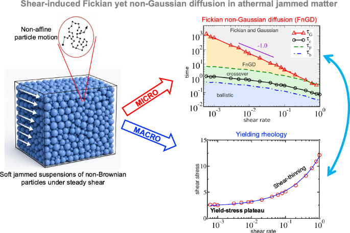
Shear-rate dependence
We start by focusing on a volume fraction ϕ = 0.68 (a value exactly in the middle of the investigated range). Figure 1a shows the MSD as a function of time for different values of the shear rate \(\dot{\gamma }\). In agreement with previous analysis on similar systems7,68, all curves display a smooth crossover from a short-time ballistic behavior, 〈r2(t)〉 = Kt2, to a long-time Fickian regime, 〈r2(t)〉 = 4Dt, as highlighted by the fits included in the figure. It is apparent that, at any given time, 〈r2(t)〉 is larger for larger shear rates, indicating that both \(K(\dot{\gamma })\) and the self-diffusion coefficient \(D(\dot{\gamma })\) increase on increasing \(\dot{\gamma }\). For each shear-rate value, the crossing of the ballistic and Fickian fits identifies a point, whose coordinates, τc and \({l}_{c}^{2}\) are analytically obtained: \({\tau }_{c}=\frac{4D}{K}\) and \({l}_{c}^{2}=\frac{{(4D)}^{2}}{K}\), being uniquely fixed by the values of K and D. τc identifies the crossover between the short-time regime dominated by directed particle motion and the long-time diffusive regime. Operationally, it corresponds to the time at which the MSD crosses over from its initial superdiffusive (ballistic-like) growth to the linear Fickian regime. The associated length lc, defined as the square root of the MSD at this time, therefore represents the typical particle displacement accumulated up to the onset of diffusion. On lowering the shear rate in the investigated range, \({\tau }_{c}(\dot{\gamma })\) increases by about a factor ten (see Fig. 1c), and \({l}_{c}(\dot{\gamma })\) increases by about a factor 3 (see Fig. S5 in Supplementary Information). Being the characteristic time and length of the ballistic-to-Fickian crossover, τc and lc naturally set an upper boundary for the extension of ballistic regime and a lower boundary for the onset of Fickian regime. Now we show that their role goes far beyond this aspect.
Fig. 1: Single-particle dynamics at fixed volume fraction and varying shear rate.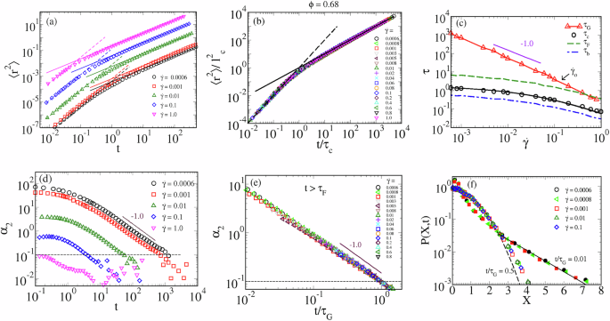
At volume fraction ϕ = 0.68: a (non-affine) MSD in x−y (Gradient-Vorticity) plane as a function of the time 〈r2(t)〉 at different shear rate \(\dot{\gamma }\), as indicated in the figure legend. Dashed and solid lines are ballistic and Fickian fits to short- and long-time data, respectively. For each \(\dot{\gamma }\), the coordinates of the crossing point identify τc and \({l}_{c}^{2}\). b MSD at different shear rates, after rescaling the axes by τc and \({l}_{c}^{2}\), respectively. Dashed and solid lines are ballistic and Fickian fits to the obtained master curve, at short- and long-time, respectively. c Time of the ballistic-to-Fickian crossover τc and Gaussian time τG as a function of \(\dot{\gamma }\). The dashed-dotted and the dashed lines parallel to τc identify the ballistic time τb = 0.4τc and the Fickian time τF = 5τc, respectively. The arrow marks the position of the shear rate \({\dot{\gamma }}_{o}\) where \({\tau }_{G}({\dot{\gamma }}_{o})=2\,{\tau }_{F}({\dot{\gamma }}_{o})\). The purple solid line is a guide to the eyes of slope − 1. The black solid line is an estimate of τc obtained by combining Eqs. (1) and (2). d Non-Gaussian parameters as a function of the time, α2(t), associated to the MSDs in panel a. The dashed line marks the position of the threshold used to define τG. e Non-Gaussian parameter after rescaling the time by τG, at different shear rates, in the Fickian regime (t≥τF). The solid lines in (d) and (e) are guides to the eyes of slope − 1. f Rescaled particle displacement distribution, P(X, t), as a function of the non-dimensional displacement length X, for two values of the non-dimensional time t/τG, at different shear rates, in the Fickian regime (t ≥ τF). The dashed line is the universal Brownian-Gaussian distribution G(X). The solid line is an exponential fit, ae−(X/Λ) with a = 0.2 and Λ = 1.3 to the tails.
To this aim, Fig. 1b shows the MSDs at different \(\dot{\gamma }\) after rescaling the horizontal and vertical coordinates by τc and \({l}_{c}^{2}\), respectively. All datasets finely collapse over a single master curve, not only in the ballistic and Fickian regimes but also across the crossover. The existence of such a robust master curve implies that any dependence of the MSD on the shear-rate is ruled uniquely by τc and lc.
The data collapse of Fig. 1b can also be exploited to define a marker for the onset of the Fickian regime, τF. Indeed, the existence of a master curve implies that this time is a fixed (\(\dot{\gamma }\)-independent) multiple of τc, with the proportionality factor depending only on the specific measurement protocol. Here, we estimate τF as the time at which the master curve starts being compatible with the long-time Fickian behavior, within the modest dispersion of the data collapse, obtaining \({\tau }_{F}(\dot{\gamma })=5{\tau }_{c}(\dot{\gamma })\) (dashed line in Fig. 1c). A similar argument holds for the duration of the earlier ballistic motion, τb, i.e. the time when the master curve ceases to be compatible with the ballistic behavior, for which we obtain \({\tau }_{b}(\dot{\gamma })=0.4{\tau }_{c}(\dot{\gamma })\) (dash-dotted line in Fig. 1c). The corresponding diffusion lengths, \(\sqrt{4D{\tau }_{F}}\) and \(\sqrt{K}{\tau }_{b}\), are likewise simply proportional to lc. We remark that these quantities are therefore not independent time and length scales, but simply operational markers proportional to the characteristic time and length of the crossover.
Next, we turn to study the NGP, α2(t), which is shown in Fig. 1d for the same \(\dot{\gamma }\) values considered in panel a. We recall that the value of α2(t) quantifies, on a cumulative level, the deviations of the PDD p(x, t) from a Gaussian distribution. Indeed, α2 is identically null for a Brownian-like diffusion process. A very different behavior is, in fact, observed in the present case. At short times, each curve stays close to a plateau, whose value increases by about two orders of magnitude on lowering \(\dot{\gamma }\). After leaving the plateau, all curves decrease monotonically with a similar slope (in log-log scale). Accordingly, at any time, the NGP is larger for smaller shear rates. At relatively long times, it is apparent that α2(t) tends to decrease approximately as t−1 (solid line in panel d). At the longest investigated times, α2(t) eventually becomes compatible with zero within the noise.
A visual comparison of panel a and d already shows that, when the MSD enters the Fickian regime, the NGP is still far from having vanished, at low shear rate at least. To quantitatively define a characteristic time τG for the recovery of Gaussianity, we try to collapse the long-time NGP decays at different \(\dot{\gamma }\), by properly rescaling the time. As a matter of fact, Fig. 1e shows that at long-time, corresponding to the Fickian regime t≥τF, all datasets finely fall over a single master curve (for an NGP plot including also shorter times, see Fig. S2 in Supplementary Information). The time-rescaling factors at different \(\dot{\gamma }\) define \({\tau }_{G}(\dot{\gamma })\), apart from a constant, which can be fixed by imposing t/τG = 1 when the master curve decreases to a given threshold. The existence of a master curve implies that the \(\dot{\gamma }\) dependence of τG is unaffected by the choice of the threshold. Here, we select a threshold of 0.1, that is slightly larger than the typical long-time noise of the NGP. (When α2(t) is always less than 0.1, as it occurs at large shear rates \(\dot{\gamma } > 0.8\), we assume \({\tau }_{G}(\dot{\gamma })={\tau }_{F}(\dot{\gamma })\), i.e., there is no FnGD).
Figure 1c shows that the so-measured \({\tau }_{G}(\dot{\gamma })\) increases much faster than \({\tau }_{c}(\dot{\gamma })\) (over four orders of magnitude) on lowering the shear rate, up to exceeding \({\tau }_{F}(\dot{\gamma })\) by a factor 100. Thus, at small shear rate, the restoring of Gaussianity occurs much later than the onset of Fickian regime, which is a clear-cut signature of the presence of SI-FnGD. Importantly, on decreasing the shear rate, τc varies only weakly in the low-\(\dot{\gamma }\) regime, even suggesting a tendency toward saturation in a low-shear-rate plateau, whereas τG keeps increasing strongly, approximately as \({\dot{\gamma }}^{-1}\). This behavior implies that the recovery of Gaussian statistics is associated with an approximately constant accumulated strain, \(\dot{\gamma }{\tau }_{G} \sim {{\rm{const}}}\), whereas the onset of diffusion is not. As a consequence, on decreasing the shear rate, the onset of diffusion remains relatively fast, while the recovery of Gaussian statistics is shifted to much longer times.
The Gaussian length ξG, defined as the square root of the MSD at τG, represents the diffusion length associated with the restoration of Gaussian displacement statistics. Accordingly, the Gaussian length \({\xi }_{G}(\dot{\gamma })=\sqrt{4D(\dot{\gamma }){\tau }_{G}(\dot{\gamma })}={l}_{c}(\dot{\gamma })\sqrt{\frac{{\tau }_{G}(\dot{\gamma })}{{\tau }_{c}(\dot{\gamma })}}\), largely exceeds the Fickian one at small shear rates.
From the data in Fig. 1c, we also estimate a shear rate \({\dot{\gamma }}_{o}\) (as indicated by the arrow) indicative of the onset of a clearly observable FnGD time window. As a matter of fact, we define \({\dot{\gamma }}_{o}\) as the shear rate where the Gaussian time becomes twice the Fickian time, \({\tau }_{G}({\dot{\gamma }}_{o})=2\,{\tau }_{F}({\dot{\gamma }}_{o})\), or equivalently \({\tau }_{G}({\dot{\gamma }}_{o})=10{\tau }_{c}({\dot{\gamma }}_{o})\). For \(\dot{\gamma }\le {\dot{\gamma }}_{o}\) the “FnGD time-window” (τG/τF) clearly enlarges.
The emergence of the timescale τG suggests that the NGPs (and in turn the underlying displacement distributions) are not uniquely controlled by the only timescale, τc, relevant for the MSDs. Indeed, we checked that it is not possible to collapse the NGPs over the whole time-window considered in panel d by rescaling time with τc (see Fig. S3 in the Supplementary Information), as previously done for the MSDs. In spite of this, we have shown that a data-collapse limited to the SI-FnGD time window can still be obtained by plotting α2(t) against t/τG.
It is thus tempting to check whether the non-dimensional time \(\frac{t}{{\tau }_{G}(\dot{\gamma })}\) also controls the overall shape of the underlying PDD functions p(x, t), at long time at least. (Of course, this is not an obvious issue, as one may expect that other timescales become relevant on considering moments of order larger than the fourth one, present in the NGP.) To this aim, we show in Fig. 1f the displacement distributions at different shear rates, in a range spanning more than three decades, and different times in the SI-FnGD time-window. To properly compare the distributions on such a wide range of times and shear rates (in turn corresponding to a broad spectrum of displacements), we have rescaled the axes as follows: \(x\to X=\frac{x}{\sqrt{\langle {x}^{2}(t)\rangle }}\), and \(p(x,t)\to P(X,t)=p(x,t)\sqrt{\langle {x}^{2}(t)\rangle }\), thus preserving normalization. Notably, after this re-scaling, the Gaussian distribution \(g(x,t)=\frac{{e}^{-\frac{{x}^{2}}{4Dt}}}{\sqrt{\pi Dt}}\) corresponding to standard Brownian motion becomes a universal, time-independent curve: \(G(X)=\sqrt{\frac{2}{\pi }}{e}^{-\frac{{X}^{2}}{2}}\). For the different \(\dot{\gamma }\) in Fig. 1f, P(X, t) is reported for times corresponding to t/τG = 0.01 and 0.5, provided that t > τF (notice that it is 0.01τG > τF only for sufficiently low shear rates, and therefore only those shear rates have been included in the figure, for t/τG=0.01). The figure shows that all datasets corresponding to the same t/τG follow the same mastercurve, regardless of \(\dot{\gamma }\). Thus, t/τG actually controls the overall shape of the displacement distribution in the SI-FnGD (over the whole probability range of our simulations, at least). Concerning the temporal evolution of the mastercurve, clear deviations from the Brownian Gaussian (dashed line) are present at the shortest non-dimensional time t/τG = 0.01. At intermediate non-dimensional displacements, P(X, t) displays a probability deficit with respect to the Gaussian distribution. This deficit is sandwiched between excess probabilities at small and large X, leading to crossings between P(X, t) and G(X, t) at X ≈ 0.5 and X ≈ 2.5, respectively. Such a double-crossing feature has also been reported in other instances of FnGD18,19 and indicates the presence of long-standing dynamical heterogeneities (i.e., populations of “fast” and “slow” particles), which persist even in the well-established Fickian regime. Non-Gaussian deviations at large X also display a benchmark typically associated to FnGD since its discovery8,9, taking the form of exponential tails, \(P(X,t)\simeq {e}^{-\frac{| X| }{{\rm\Lambda }}}\), where Λ is a non-dimensional decay length. We note that, although more complex functional forms may provide better descriptions of the tails 36, the exponential form is often used in this context as an operational choice, since it captures the tail behavior reasonably well over the accessible dynamic range with a minimal number of fitting parameters9. As time goes on, non-Gaussian deviations are expected to disappear and to become almost undetectable on approaching τG. Indeed, Fig. 1f shows that, at the longest non-dimensional time t/τG = 0.5, the master curve of P(X, t) has almost reverted to G(X, t), with slight deviations persisting only in the tails.
Overall, these results confirm that the Gaussian recovery is controlled by a timescale \({\tau }_{G}(\dot{\gamma })\) distinct from the one \({\tau }_{c}(\dot{\gamma })\) governing the ballistic-to-Fickian crossover.
Volume fraction dependence
We now turn to discussing how the above-presented features change with the volume fraction. On varying ϕ in the considered range [0.58, 0.78], the MSD and NGP do not show qualitative changes with respect to the behaviors presented in Fig. 1a, d for ϕ = 0.68. However, the characteristic time and length of the ballistic-to-Fickian crossover, τc and lc, and the Gaussian time τG are all found to depend, not only on the shear rate, but also on the volume fraction (see Figs. S4 and S5 in Supplementary Information). \({\tau }_{c}(\dot{\gamma },\phi )\) and \({l}_{c}(\dot{\gamma },\phi )\) corresponding to different ϕ show a similar \(\dot{\gamma }\) dependence, but their values decrease with increasing ϕ (over a range comparable to that observed as function of \(\dot{\gamma }\)), consistent with the expectation that the ballistic regime narrows as nearest-neighbor particles get closer. On the other hand, \({\tau }_{G}(\dot{\gamma },\phi )\), shows a slight increase with the volume fraction, which is almost negligible if compared to the variations of orders of magnitude observed as a function of the shear rate. The resulting shear rate \({\dot{\gamma }}_{o}\) for the onset of FnGD is also found to increase by a factor ≃ 4 on increasing ϕ. In Fig. 2a, b, c, we have plotted MSDs, NGPs and displacement distributions, respectively, after rescaling the axes by \({\tau }_{c}(\dot{\gamma },\phi )\), \({l}_{c}^{2}(\dot{\gamma },\phi )\), \({\tau }_{G}(\dot{\gamma },\phi )\) as we did in Fig. 2a and d, but now also including the volume fractions ϕ = 0.58 and 0.78. A very robust data-collapse is observed for any combination of \(\dot{\gamma }\) and ϕ, for both MSD, NGP, as well as for p(X, t) at given non-dimensional time. These results indicate how the previously identified master curves are somewhat “universal”, as they describe the dynamics not only at different shear rates but also at different volume fractions. As a consequence, the conclusions drawn for the dependence on the shear-rate can now be extended to the volume fraction. Accordingly, for instance, \({\tau }_{c}(\dot{\gamma },\phi )\) and \({l}_{c}(\dot{\gamma },\phi )\) control the dependence of any MSD-derived properties on both ϕ and \(\dot{\gamma }\), including D, K, τF, τB. Similarly, in the SI-FnGD regime, the value of NGP and of the overall displacement distribution at different \(\dot{\gamma }\) and ϕ are still controlled uniquely by \(\frac{t}{{\tau }_{G}(\dot{\gamma },\phi )}\).
Fig. 2: Master curves of single-particle dynamics across shear rates and volume fractions.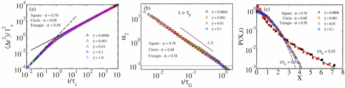
At different shear rates \(\dot{\gamma }\) and volume fractions ϕ, as indicated in the figure legends: a MSD after rescaling the axes by the crossover time and squared length, τc and \({l}_{c}^{2}\), respectively. The dashed and solid lines are ballistic and Fickian fits to the resulting master curve at short and long times, respectively. b Non-Gaussian parameter after rescaling the time by the Gaussian time τG, in the Fickian regime (t ≥ τF). The dashed line marks the position of the threshold used to define τG. The solid line is a guide to the eye with slope −1. c Rescaled particle displacement distribution, P(X, t), as a function of the dimensionless displacement X, for two values of the dimensionless time t/τG in the Fickian regime (t ≥ τF). The dashed line is the universal Brownian-Gaussian distribution G(X). The solid line is an exponential fit, ae−X/Λ with a = 0.2 and Λ = 1.3, to the tails.
Yielding and SI-FnGD
Next, we take advantage of the dynamical features described above to suggest some new perspectives on the rheology of the system. To this aim, we consider the rheological flow curves that relate the shear stress σ, measured under steady-state conditions, to the shear rate \(\dot{\gamma }\). At volume fraction well below jamming, the flow curves exhibit a Newtonian-like behavior \(\sigma \propto \dot{\gamma }\), as illustrated in the inset of Fig. 3a for ϕ = 0.40. Conversely, the flow curves shown in the main panel of Fig. 3a for three different volume fractions ϕ = 0.58, 0.68, and 0.78 above jamming, share the qualitative features reported for a wide variety of soft solids73,74. At low shear rate, the stress attains a plateau that identifies the dynamic yield stress and is found to increase with ϕ. At larger shear rate, the stress positively departs from the plateau in a sub-linear fashion, indicative of a shear-thinning regime.
Fig. 3: Linking macroscopic rheology and single-particle dynamics.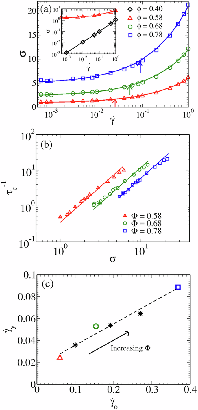
a Shear stress σ as a function of the shear rate \(\dot{\gamma }\) at three different volume fractions ϕ, as indicated in the figure legend. Solid lines are fits to the model in Eq. (1). The arrows indicate the critical shear rate \({\dot{\gamma }}_{y}\) for each ϕ. Inset: comparison between a flow curve at a volume fraction well below jamming, ϕ = 0.40, and the one at ϕ = 0.58 (also reported in the main panel). b Inverse crossover time \({\tau }_{c}^{-1}\) versus the shear stress σ at three different volume fractions, as indicated. Solid lines are quadratic fits \({\tau }_{c}^{-1}=b{\sigma }^{2}\), with b = 0.35, , 0.12, , 0.06, respectively. c \({\dot{\gamma }}_{y}\) versus the onset shear rate of FnGD, \({\dot{\gamma }}_{o}\); the volume fractions in panel a are indicated with the same symbols. Stars correspond to additional volume fractions, ϕ = 0.64, 0.70, 0.74. The dashed line is a linear fit to the data.
For each volume fraction, we find that the flow curves are well fitted by the law:
$$\sigma (\dot{\gamma },\phi )={\sigma }_{y}(\phi )\left[1+\frac{{\dot{\gamma }}^{1/2}}{{\dot{\gamma }}_{y}^{1/2}(\phi )}\right],$$
(1)
proposed by Bocquet et al.50 drawing on a previous mean-field (mode-coupling) model, where local stress relaxation, close to yielding, is driven by plastic rearrangements75.
Notice that, at variance with other rheological model for yield stress-fluids, such as the popular Herschel-Bulckley law76, Eq. (1) has the advantage of featuring only two fitting parameters: σy is the aforementioned dynamic yield stress and \({\dot{\gamma }}_{y}\) is a characteristic shear rate associated to the crossover between the yield-stress and the shear-thinning (or plastic-dissipation-dominated50) regimes. Similarly to σy(ϕ), the value of \({\dot{\gamma }}_{y}(\phi )\) is also found to increase with the volume fraction, as indicated by the arrow in Fig. 3a.
Exploring possible connections between overall rheology and microscopic dynamics, we first consider the dependence of the crossover time τc on the shear stress. Figure 3b shows that, at all investigated volume fractions, the inverse crossover time is well described by the relation:
$${\tau }_{c}^{-1}(\dot{\gamma })\propto {\sigma }^{2}(\dot{\gamma })$$
(2)
with a proportionality factor that depends only on the volume fraction. The black solid line in Fig. 1c, obtained by combining Eqs. (1) and (2), further supports the effectiveness of the latter relation in describing the data. Thus, the shear-rate dependence of τc appears to mirror that of the shear stress. In particular, the tendency of the stress to approach a plateau at low shear rates, \(\dot{\gamma } < {\dot{\gamma }}_{y}\), is directly reflected in the behavior of \({\tau }_{c}(\dot{\gamma })\). By contrast, as already anticipated by the collapse of the NGP and PDD, the Gaussian time is found to scale approximately as \({\tau }_{G}(\dot{\gamma })\propto {\dot{\gamma }}^{-1}\), implying that the recovery of Gaussianity is associated with an approximately constant accumulated strain, unlike the onset of Fickian diffusion. Thus, the increasing separation between τc and τG and the resulting emergence of SI-FnGD appear to be related to the “decoupling” between shear stress and shear rate in the flow curve, which marks the onset of yielding rheology.
Next, we show in Fig. 3c a scatter plot of the critical shear rate from rheology \({\dot{\gamma }}_{y}(\phi )\) versus the characteristic shear rate \({\dot{\gamma }}_{o}(\phi )\) for the onset of SI-FnGD, as measured at different volume fractions. The onset of SI-FnGD appears to be strongly correlated with the onset of yielding rheology. In fact, data are compatible with an approximately linear relation between the two shear rates, whose values are also of the same order of magnitude. This result can be rationalized in the light of the behavior discussed above. At large shear rates, \({\tau }_{F}(\dot{\gamma })\simeq {\tau }_{G}(\dot{\gamma })\). At smaller shear rates τG increases approximately as \({\dot{\gamma }}^{-1}\), whereas \({\tau }_{F}(\dot{\gamma })\propto {\sigma }^{-2}(\dot{\gamma })\) shows a tendency toward a plateau around \({\dot{\gamma }}_{y}\), like the stress does. Thus, \({\dot{\gamma }}_{y}\) is also the shear rate where τG starts to decouple from τF. Accordingly, \({\dot{\gamma }}_{o}\), defined as the shear rate below which SI-FnGD becomes clearly observable in terms of its time-window, τG/τF, is expected to lie close to \({\dot{\gamma }}_{y}\).
Heterogeneous Persistent Random Walk frameworkOverview
In the following, we introduce a minimal model aimed at capturing the main features observed in our system. We refer to this framework as a Heterogeneous Persistent Random Walk (HPRW). This framework combines ideas from Persistent Random Walk (PRW)77,78,79 with concepts that underlie several models of FnGD, such as superstatistics and diffusing-diffusivity approaches9,34,35,36,37,38.
We start from the observation that the ballistic-to-Fickian MSD crossover of our system naturally recalls a PRW. At the same time, given the marked heterogeneity typical of soft amorphous solids, the system can be viewed, at a coarse-grained level, as composed of different local domains, each characterized by its own local properties (including dynamical ones)61,80. Thus, our HPRW framework rests on the assumption that, for times t ≪ τG, each particle performs a PRW within its initial domain. Heterogeneity is encoded in the fact that different domains have different characteristic persistence times τpj, distributed over domains according to a control-parameter-dependent function \(P({\tau }_{pj};\dot{\gamma },\phi )\). For the sake of simplicity, we assume the particle speed \(v(\dot{\gamma },\phi )\) to be uniform and to depend only on the external control parameters. Accordingly, the characteristic persistence length in domain j is \({l}_{pj}=v(\dot{\gamma },\phi ){\tau }_{pj}\), so that its distribution is fully determined by \(P({\tau }_{pj};\dot{\gamma },\phi )\). (For the sake of conciseness, in the following we will omit the explicit dependence on the external control parameters, \(\dot{\gamma },\phi\) and ϕ, whenever it is not strictly necessary).
Next, we consider that, because of the imposed shear and the ensuing structural rearrangements, the local environment experienced by a particle is renewed over a finite timescale, reflecting, in our view, both a finite lifetime of domains and the possibility for particles to escape their initial domain. Our minimal description assumes that this timescale is of order τG, with the rheologically meaningful implication that the local environment is renewed after an approximately shear-rate-independent strain \(\sim \dot{\gamma }{\tau }_{G}\), consistent with the observed scaling \({\tau }_{G}\propto {\dot{\gamma }}^{-1}\). Hence, for times of order τG, a particle has explored different domains, effectively sampling the distribution of τpj.
MSD behavior
The MSD of particles moving within a given domain j, \(\langle {r}_{j}^{2}(t)\rangle\), follows the standard PRW behavior. Accordingly, for t ≪ τpj one has ballistic motion, \(\langle {r}_{j}^{2}(t)\rangle ={v}^{2}{t}^{2}\), whereas for t ≳ τpj the MSD crosses over to the Fickian form \(\langle {r}_{j}^{2}(t)\rangle =4{D}_{j}t\), which is typically established within a few persistence times τpj. Here the domain diffusivity is Dj = v2τpj/2. Thus, while the short-time ballistic prefactor is common to all domains, the long-time diffusivity depends on the local persistence time and is therefore domain-dependent.
The overall measured MSD is obtained by averaging the single-domain contributions over the distribution of persistence times (assuming the unit normalization of the distribution). In the ballistic regime, one simply has
$$\langle {r}^{2}(t)\rangle =\int\,P({\tau }_{pj})\,{v}^{2}{t}^{2}\,d{\tau }_{pj}={v}^{2}{t}^{2},$$
(3)
since the short-time behavior is the same in all domains. Once the relevant single-domain PRWs are in their Fickian regime, one instead finds
$$\langle {r}^{2}(t)\rangle =\int\,P({\tau }_{pj})\,2{v}^{2}{\tau }_{pj}\,t\,d{\tau }_{pj}=2{v}^{2}{\tau }_{p}\,t,$$
(4)
where \({\tau }_{p}={\langle {\tau }_{pj}\rangle }_{j}=\int\,P({\tau }_{pj}){\tau }_{pj}\,d{\tau }_{pj}\) is the average persistence time over domains (similarly, we denote with \({l}_{p}={\langle {l}_{pj}\rangle }_{j}=v{\tau }_{p}\) the average persistence length). Equivalently, \(\langle {r}^{2}(t)\rangle =4{\langle {D}_{j}\rangle }_{j}\,t\), where \({\langle {D}_{j}\rangle }_{j}=\int\,P({D}_{j}){D}_{j}\,d{D}_{j}={v}^{2}{\tau }_{p}/2\) is an average diffusivity and P(Dj) the diffusivity distribution over domains9,35,36. Therefore, the overall MSD remains consistent with that of a PRW, with an effective persistence time and diffusivity given by the corresponding averages over domains. A comparison between the HPRW predictions of Eqs. (3) and (4) and the MSD of Fig. 1 leads to identify K = v2 and the diffusion coefficient \(D={\langle {D}_{j}\rangle }_{j}\), where these quantities generally depend on the control parameters \((\dot{\gamma },\phi )\). It then follows that τp = 2D/K = τc/2 and \({l}_{p}=2D/\sqrt{K}= {l}_{c}/2\). Thus, the average persistence time and length, τp and lp, of the HPRW framework act as proxies for the measured crossover time and length, τc and lc. We also notice that the measured values τb = 0.4τc and τF = 5τc, which bound the ballistic-to-Fickian crossover, can also be viewed as approximate lower and upper bounds for the relevant range of persistence times, their separation being consistent with a relatively wide distribution P(τpj).
As a further point, Eqs. (3) and (4) imply that, upon changing control parameters, the MSD follows the same master curves in both the ballistic and Fickian regimes if the axes are rescaled by \({\tau }_{p}(\dot{\gamma },\phi )\) and \({l}_{p}^{2}(\dot{\gamma },\phi )\) (or equivalently by \({\tau }_{c}(\dot{\gamma },\phi )\) and \({l}_{c}^{2}(\dot{\gamma },\phi )\)), consistently with the data collapse observed in Figs. 1b and 2a. Beyond this, the fact that the collapse also includes the crossover between the asymptotic regimes strongly suggests that \(P({\tau }_{pj};\dot{\gamma },\phi )={\tau }_{p}^{-1}f({\tau }_{pj}/{\tau }_{p})\), with the distribution f of the reduced persistence time τpj/τp remaining invariant. In this sense, the effect of the control parameters is entirely encoded in the average persistence time \({\tau }_{p}(\dot{\gamma },\phi )\). We also note that, for the standard PRW with an exponential persistence-time distribution, the velocity autocorrelation function is analytically known. Hence, if the intra-domain dynamics follow a standard PRW, the HPRW crossover in the MSD can be described in terms of that velocity autocorrelation function averaged over domains.
PDD behavior and emergence of FnGD
Within the standard PRW model, the PDD becomes Gaussian once the Fickian regime is reached. Accordingly, for t ≳ τpj, the local PDD in a given domain j reads \({p}_{j}(x,t)=\exp [-{x}^{2}/(4{D}_{j}t)]/\sqrt{4\pi {D}_{j}t}\).
By contrast, within the HPRW framework, the overall PDD can remain non-Gaussian even when the overall MSD is already Fickian, provided that the persistence time and the local-environment renewal time are well separated, namely τp ≪ τG. Indeed, for times τp ≲ t ≪ τG, each particle still moves within its initial domain, so that the PDD is obtained as a superposition of Gaussian propagators with different diffusivities:
$$p(x,t)=\int\,P({D}_{j})\frac{\exp \left(-\frac{{x}^{2}}{4{D}_{j}t}\right)}{\sqrt{4\pi {D}_{j}t}}\,d{D}_{j}.$$
(5)
Thus, local Gaussianity does not imply global Gaussianity. In fact, this expression is well known to yield exponential-like tails over larger ranges as the diffusivity distribution P(Dj) becomes wider9,35. Therefore, within the HPRW framework, FnGD arises naturally from a distribution of diffusivities, which is in turn induced by a distribution of persistence times.
We also notice that, if the distribution of reduced persistence times is independent of the control parameters, then the corresponding distribution of reduced diffusivities Dj/D is independent of them as well. Using this condition in Eq. (5), it follows that, for times τp ≲ t ≪ τG (i.e., in the early FnGD regime), the rescaled displacement distribution P(X, t) becomes independent of the control parameters, consistently with the collapse observed in Figs. 1f, 2c for t/τG = 0.01.
Long-time Gaussian recovery
At longer times, as t becomes of order τG, the assumption that each particle keeps the diffusivity of its initial domain breaks down. In this regime, a particle progressively explores different domains and therefore samples different values of the local diffusivity Dj. A useful way to rationalize this evolution is in terms of the number of statistically independent domains explored by a particle over a time t. In our picture, we assume that this number scales as n(t) ∝ t/τG. Accordingly, in this time range the quantity controlling the single-particle displacement statistics is no longer the diffusivity of the initial domain, Dj, but rather an effective diffusivity Deff(t), defined as the temporal average of the local diffusivity along the trajectory. Deff(t) → D is expected at long times, due to self-averaging.
Since the trajectory can be coarse-grained in n(t) segments with statistically independent diffusivities, the variance of Deff(t) decreases as the inverse of n(t), namely:
$${{\rm{Var}}}[{D}_{{{\rm{eff}}}}(t)]=\frac{{{\rm{Var}}}({D}_{j})}{n(t)}\propto {\left(\frac{t}{{\tau }_{G}}\right)}^{-1}.$$
(6)
The corresponding distribution Pt(Deff) can still be connected to the displacement distribution through a straightforward generalization of Eq. (5): \(p(x,t)=\int\,{P}_{t}({D}_{{{\rm{eff}}}})\frac{\exp \left[-\frac{{x}^{2}}{4{D}_{{{\rm{eff}}}}t}\right]}{\sqrt{4\pi {D}_{{{\rm{eff}}}}t}}\,d{D}_{{{\rm{eff}}}}.\) For t ≪ τG, one has Deff(t) ≃ Dj (for a particle initially belonging to domain j), so that Pt(Deff) reduces to the initial diffusivity distribution P(Dj) entering Eq. (5). At longer times, instead, the progressive narrowing of Pt(Deff) drives the recovery of Gaussianity, consistently with the observed behavior on times of order τG.
This picture also helps rationalize the collapse of P(X, t) at relatively long times, as observed in Figs. 1f and 2c for t/τG = 0.5. Indeed, if (i) the exploration of domains is controlled by t/τG and (ii) the initial distribution P(Dj) is the same upon rescaling with the average diffusivity D (as discussed above), then the long-time evolution of the displacement statistics is also expected to depend only on t/τG. Thus, the collapse of P(X, t) at different shear rates and volume fractions is expected to persist, at fixed non-dimensional time t/τG, also in the late stage of the FnGD regime.
Finally, within this framework, the NGP can be directly related to the distribution of the effective diffusivity Deff(t). Indeed, it is〈x2(t)〉 = 2〈Deff(t)〉t = 2Dt and \(\langle {x}^{4}(t)\rangle =12\langle {D}_{{{\rm{eff}}}}^{2}(t)\rangle {t}^{2}\), so that the one-dimensional NGP reads \({\alpha }_{2}(t)=\frac{\langle {x}^{4}(t)\rangle }{3{\langle {x}^{2}(t)\rangle }^{2}}-1=\frac{\langle {D}_{{{\rm{eff}}}}^{2}(t)\rangle }{{\langle {D}_{{{\rm{eff}}}}(t)\rangle }^{2}}-1=\frac{{{\rm{Var}}}\left[{D}_{{{\rm{eff}}}}(t)\right]}{{\langle {D}_{{{\rm{eff}}}}(t)\rangle }^{2}}\). This result can be straightforwardly generalized to higher dimensions. Therefore, the decay of the NGP at long times directly reflects the progressive reduction of the fluctuations of the effective diffusivity and, using Eq. (6), one finally obtains \({\alpha }_{2}(t)\propto {\left(\frac{t}{{\tau }_{G}}\right)}^{-1}\), in agreement with the behavior observed in Figs. 1e and 2b.