
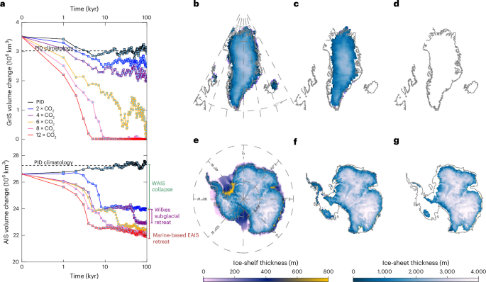
Coupled atmosphere–ocean–ice-sheet model
To determine the long-term evolution of the polar ice sheets to various CO2 forcings, we coupled the CESM1.226 and three-dimensional ice-sheet–ice-shelf PSUIM27 (Supplementary Fig. 1), using an asynchronous coupled method28. The coupled model will be referred to as CPIM1. The CESM1.2 model is based on the CAM4 atmosphere model (T31, ~3.75° resolution, 26 vertical levels), the POP2 ocean model (gx3v5, 100 × 116 horizonal grids and 25 vertical levels), CLM4.0 land physics (T31, prescribed vegetation) and the CICE4 (gx3v5, Los Alamos sea ice model) sea ice components. The CESM configuration of our coupled CPIM1 simulations is identical to the setup described in a recent study43, including the model version (CESM1.2), horizontal resolution and physical parametrizations. This setup was shown to reproduce realistic large-scale temperature and precipitation patterns under palaeoclimate CO2 forcing, supporting its adequacy for providing polar climate forcing relevant to ice-sheet studies. Despite the relatively coarse resolution, our model is able to capture the large-scale circulation features, including the Atlantic Meridional Overturning Circulation and other key phenomena (Extended Data Fig. 6 and Supplementary Fig. 13). The PSUIM represents the land ice-sheet–ice-shelf components for both the Northern Hemisphere (1.0° longitude × 0.5° latitude resolution) and the Southern Hemisphere (a stereographic grid with a 20-km resolution). Its performance has been described in recent studies15,30,44,45, demonstrating that the model reproduces key dynamical features of ice-sheet evolution, including nonlinear sensitivity and associated sea-level contributions across both hemispheres and a range of palaeo and future climate forcings, supporting the suitability of PSUIM for long-term ice-sheet sensitivity experiments.
In the asynchronously coupled ice–climate framework, we integrated CESM for 10 years and PSUIM for 1,000 years in each coupling cycle, corresponding to a climate acceleration factor of 100 (defined as the ratio of CESM to PSUIM integration lengths). The coupling frequency between CESM and PSUIM is set to 1,000 years, achieved by applying the CESM-simulated climate of monthly surface air temperature, precipitation, surface shortwave radiation and annual mean 400-m subsurface ocean temperature to PSUIM. Subsequently, CESM is forced in return for 10 years by PSUIM-simulated ice-sheet cover, topography, surface roughness and freshwater fluxes. Specifically, the surface geopotential (PHIS) and topographic standard deviation (SGH) fields in CAM4, together with ice-covered surface conditions (for example, PCT_GLACIER) in CLM4.0, are updated at each coupling time step so that CESM experiences the effect of the evolving ice-sheet topography and associated surface changes.
The coupled model uses a simplified bias correction approach for temperature and precipitation, using the ERA-5 reanalysis46 and Levitus ocean data47. Present-day climatological atmosphere and ocean temperature biases are corrected additively on the basis of differences from observations (anomaly-based correction), whereas precipitation biases are corrected multiplicatively using scaling factors derived from observations (Supplementary Fig. 14). The surface air temperature and precipitation from CESM are further downscaled to the high-resolution topography of PSUIM with lapse-rate corrections (γ = 5 °C km−1) and elevation–desertification correction. In the ocean, the model interpolates modern annual mean ocean temperatures at a depth of 400 m onto the ice-sheet model grid. In areas outside the spatial coverage of the ocean model grid, ocean temperatures are propagated beneath the ice shelves using a nearest-neighbour interpolation. The freshwater forcing from PSUIM runoff is applied to the CESM ocean grid cells along the ice-sheet perimeter and prescribed as virtual salinity fluxes to conserve ocean mass (therefore, sea level does not change explicitly in this setup of POP2). The liquid runoff (for example, basal melt and surface runoff) is routed directly to the nearest ocean grid points. Solid icebergs are considered as free-floating chunks of ice. They can drift and melt elsewhere, so the solid runoff (for example, calving of icebergs and cliff failure) from Northern Hemisphere and Southern Hemisphere ice sheets is converted into a homogeneous surface flux spread over the North Atlantic (50° N–70° N) and the Southern Ocean (poleward of 60° S). Although our coupled framework includes meltwater–ocean interactions, specific short-term feedbacks, such as meltwater-induced subsurface ocean warming and the amplification of subshelf melting48, are not explicitly isolated in the long-term diagnostics. This reflects the use of an asynchronous coupling strategy with 1,000-year ice–climate exchange intervals, a modelling choice intended to investigate millennial-scale ice-sheet responses rather than transient decadal feedbacks.
PUSIM parametrizations
The PSUIM calculates the surface mass and energy balances on the basis of the insolation–temperature melt model49. The net surface energy balance is calculated by the simplified equation:
$${{\rm{d}}E}=\left(1-\alpha \right)Q+10T-m$$
(1)
This includes the surface incoming shortwave radiation (first term, where Q is surface insolation and α is surface albedo) and a linear parametrization of the longwave radiation and turbulent heat exchanges (second term, where T is the daily mean temperature and m is a constant parameter). The parameter m was set here to 45 W m−2 in both Northern and Southern Hemispheres. The offline PSUIM also includes representations of the lapse-rate corrections (γ = 5 °C km−1) and elevation–desertification process due to atmospheric drying (CC factor of \({2}^{\frac{-\gamma \triangle H}{10\circ c}}\)) and parametrizations of calving hydrofracturing and marine ice-cliff failure, as well as inverse-derived basal sliding coefficients27,50. The CPIM1 in our study uses the same script-based, flexible coupling technique as the intermediate complexity model LOVECLIM–PSUIM15,30. In the coupling framework, the climate and ice-sheet models are run sequentially and linked through externally controlled coupling scripts. CESM-derived climate forcing is downscaled onto the higher-resolution PSUIM grid. Whereas CESM resolves melt by explicitly solving the full surface energy balance (including net radiation, latent and sensible heat fluxes), the surface mass balance in our simulation is calculated within PSUIM using a simple insolation–temperature melt scheme. Rain–snow partitioning is likewise diagnosed internally as a function of surface temperature. This approach allows surface mass balance to respond consistently to evolving, high-resolution ice-sheet topography within the ice model, while retaining the dominant thermodynamic controls on melt.
The PSUIM does not explicitly resolve ocean circulation within ice-shelf cavities and instead represents sub-ice-shelf forcing through parametrized basal melt rates. Basal melting rates are calculated using a quadratic dependence on thermal forcing27, defined as the difference between the 400-m subsurface ocean temperature (TO; K) and the local freezing point temperature at a given depth (Tf). The resulting ocean-driven melt rate (OM) is given by:
$${\rm{OM}}=\frac{{O}_{\rm{melt}}{K}_{\rm{T}}{\rho }_{\rm{w}}{c}_{\rm{w}}}{{\rho }_{\rm{i}}{L}_{\rm{f}}}\left|({T}_{\rm{O}}-{T}_{\rm{f}})\right|({T}_{\rm{O}}-{T}_{\rm{f}})$$
(2)
where Omelt, KT, cw, ρw and ρi denote the oceanic melting parameter (Omelt = 1.0), transfer coefficient for sub-ice oceanic melting (15.77 m yr−1 K−1), specific heat of ocean water (4,218 J kg−1 K−1), density of ocean water and ice (1,028 kg m−3 and 910 kg m−3), respectively. We used a subsurface reference depth of 400 m to represent subsurface thermal forcing relevant for basal melting, consistent with previous studies6,51, as this depth broadly captures the level at which relatively warm subsurface waters interact with ice-shelf bases. The use of a fixed 400-m thermal forcing is a simplification, particularly for WAIS sectors where the grounding line deepens during retreat and may increasingly interact with warmer circumpolar deep waters. The 400 m simplification may, therefore, delay the timing of the grounding-line retreat and transient ice mass loss responses. However, given the multimillennial timescales in the present study and the vertically rather homogenous subsurface warming (~300–700 m) in the simulations (Supplementary Fig. 15), the main conclusions regarding long-term ice-sheet sensitivity are unlikely to depend on the choice of reference depth. Grounded basal melt is controlled by the basal energy budget, with melting occurring when combined geothermal heat flux and frictional heat inputs surplus conductive heat transfer through the ice.
Ice-shelf calving occurs when surface and basal crevasses extend sufficiently to approach full-thickness penetration of the ice column. The model represents additional calving processes associated with hydrofracturing driven by surface meltwater and rainfall, as well as failure of tall ice cliffs linked to marine ice-cliff instability (MICI). The resulting penetration depth of water-filled crevasses, dw (m), is defined as:
$${d}_{\rm{w}}={\rm{CREVLIQ}}\,{R}^{2}$$
(3)
where CREVLIQ is set to 100 m−1 yr2 and R is the annual surface meltwater and rainfall (m yr−1). The MICI parametrization is applied with a maximum horizonal ice-cliff wastage rate (VCLIF) of 3 km yr−1.
Glacial isostatic adjustment is represented using the elastic lithosphere–relaxing asthenosphere framework, assuming a spatially uniform flexural rigidity of 1025 N m, a bedrock density of 3,370 kg m−3 and a single mantle relaxation timescale of 3,000 years. Although this simplified treatment reproduces the effect of bed deformation induced by ice and ocean loading, it does not account for lateral variations in mantle viscosity. The grounding-line migration is determined by local flotation conditions: the grounding line retreats when ice thins to flotation and advances when ice thickens above flotation27. Ice flux across the grounding line is calculated using the Schoof flux parametrization52. This formulation permits dynamic grounding-line advance and retreat in response to evolving ice thickness, without requiring explicit front tracking. The hemispheric interactions are controlled through global sea-level change. Changes in eustatic sea level, computed from the combined bihemispheric ice-sheet volumes, influence ice-shelf dynamics by modulating the grounded and floating ice fluxes at the grounding line. The SLE changes are calculated using the standard volume-above-flotation approach, accounting for evolving bedrock topography and sea-level forcing, but without additional ocean volume or density corrections53.
Ice dynamics are computed using a hybrid shallow-ice–shallow-shelf stress balance, with the shallow-ice approximation applied to grounded ice and the shallow-shelf approximation governing fast-flowing ice streams and floating ice shelves. Basal sliding is represented using a nonlinear stress–velocity relationship27, with spatially varying sliding coefficients. The sliding coefficients depend on homologous basal temperature and implicitly account for the effects of basal hydrology and substrate properties. In the Southern Hemisphere, sliding coefficients are obtained through a simplified inverse approach and constrained to the range from 10−10–10−5 m yr−1 Pa−2. In the Northern Hemisphere, a binary sliding scheme is adopted, assigning higher sliding values (10−6 m yr−1 Pa−2) to deformable marine sediments and lower values (10−10 m yr−1 Pa−2) to rigid continental bedrock30. The basal sliding coefficients are held fixed during the transient simulations, which represents a limitation of our approach and may preclude a more realistic representation of basal processes. Additional details of the PSUIM model configuration are described in a previous study27.
Coupled climate–ice-sheet sensitivity experiments
The coupled model is initialized independently in the climate and ice-sheet components. The climate component is branched after 2,300 years of a PID CESM1.2 control run, which serves as the initial condition for all PID and CO2 sensitivity experiments. In contrast, the ice-sheet initial state is taken from a previously published, quasi-equilibrated 8,000-year LOVECLIM–PSUIM simulation15. These spin-up simulations exhibit minimal long-term drift in both climate and ice volume under fixed PID forcing (Supplementary Fig. 16). Our simulations are then integrated for 100,000 years with constant CO2 forcing, allowing for the quasi-equilibration of all climate system components. To reduce computing time, we applied a climate acceleration factor of 100 to the CESM run, compressing the simulation time to 1,000 years in CESM (compared with 100,000 years in PSUIM). The PID control simulation is performed with atmospheric CO2 concentration of ~285 ppm (PID level). The warming simulations (CO2 sensitivity experiments) also apply constant CO2 values (2 × CO2, 4 × CO2, 6 × CO2, 8 × CO2 and 12 × CO2, relative to the PID condition) (Supplementary Table 1). Owing to the 1,000-year coupling frequency, the climatic conditions and ice volumes from sensitivity experiments are averaged over 1,000 years. Unless otherwise noted, results from the last 10 kyr of each sensitivity simulation are averaged and expressed as anomalies relative to the PID control mean. Statistical significance is assessed using two-sided t-tests (100 samples for PID and 10 samples for each sensitivity simulation). Using the PID climatological mean ensures a consistent reference for comparing spatial patterns across experiments, with results insensitive to the use of the PID end-state instead (Supplementary Fig. 17).
On long timescales, the climate and ice-sheet responses are primarily driven by sustained CO2 forcing rather than by transient adjustments to small perturbations in the initial conditions. We also ignore orbital changes in insolation due to the dominant Milankovitch cycles. Accordingly, instead of adopting an ensemble approach, we conducted a suite of additional sensitivity simulations to assess the robustness of our results to key model parameters and coupling choices. Lapse-rate-based precipitation corrections can substantially influence melt–elevation feedbacks, with sensitivities potentially depending on model configuration and coupling framework details54. Although hydrofracturing and MICI parametrizations are included to capture plausible high-end calving responses under extreme climate forcing, these processes remain uncertain55.
Sensitivity experiments explore the effects of (1) atmospheric parametrizations applied to the ice sheet, including precipitation correction and a lapse rate of 8 °C km−1 (Supplementary Fig. 18), (2) ocean related parameters controlling hydrofracturing (CREVLIQ = 100) and MICI (VCLIF = 0), as well as basal ocean melting rates (that is, Omelt = 2.0; Supplementary Fig. 12), (3) initial ice-sheet geometry (Supplementary Fig. 19) and (4) ice–climate coupling frequency (Supplementary Fig. 20). The experiments indicate that lapse-rate-based precipitation corrections can substantially influence melt–elevation feedbacks (Supplementary Fig. 18). In particular, a larger lapse-rate correction (8 °C km−1) produces a greater reduction in AIS volume through enhanced elevation-dependent warming. Ocean-parameter sensitivity experiments show more rapid ice loss under enhanced basal melting, whereas hydrofracturing and MICI parametrizations lead to additional AIS loss (Supplementary Fig. 12). Variations in the initial ice-sheet geometry produce only modest differences in the simulated response (Supplementary Fig. 19). In addition, simulations using shorter coupling intervals without climate acceleration and longer CESM integration periods (reducing the climate acceleration to 10) exhibit faster early-stage ice loss due to more rapid ocean adjustment, while the final ice-sheet states remain very similar to those obtained in the default configuration (Supplementary Fig. 20). All parameter sensitivities show comparable results.
Standalone ice-sheet sensitivity experiments
To examine the respective effects of insolation and precipitation sensitivity on ice viability, we performed standalone ice model simulations using climate forcing from the coupled climate–ice model run with a 12 × CO2 concentration (12CO2_L8; using the lapse rate of 8 °C km−1), the results of which are shown in Fig. 6. One ice model offline simulation applied the same configuration as the coupled run, including identical precipitation and insolation changes (ΔP and ΔS). Other offline simulations used the same configuration, but without explicit changes in insolation (ΔS = 0), precipitation (ΔP = 0) or both (ΔS = 0 and ΔP = 0).
Precipitation sensitivity to temperature changes
Precipitation sensitivity to temperature changes is quantified using two different diagnostics. At continental and ice-sheet scales, sensitivity is estimated from the regression slope between precipitation and surface air temperature anomalies (dP/dT, regression-based sensitivities; Extended Data Fig. 3). At the local grid scale, spatial patterns of sensitivity are quantified separately for each CO2 experiment using the differences between the CO2 and PID experiments, defined as ΔP/ΔT (local precipitation sensitivities; Supplementary Figs. 8,9c and 10c and Extended Data Fig. 4). Here precipitation anomalies are expressed as percentage changes relative to the PID mean, such that both estimates are shown in % K−1 to facilitate comparison with CC scaling. The temperature and precipitation changes are also examined at representative local sites over the GrIS (North Greenland Ice Core Project site; 75° N, 42° W) and WAIS (WAIS Divide site; 79° S, 112° W) and EAIS (Dome Fuji site, 77.32° S, 39.7° E).
Thermodynamic and dynamic contributions to precipitation
We calculate (1) the total relative precipitation change in the 12 × CO2 experiment relative to PID (ΔP; %), (2) the one related to the CC thermodynamic contribution (ΔPT) and (3) the dynamic contribution to precipitation (ΔPdyn) (Fig. 4). The thermodynamic changes are simply calculated as follows33,56:
$$\Delta {P}_{\rm{T}}={M}^{* }\Delta {q}_{\rm{cc}}$$
(4)
where M* is the PID ratio of precipitation to specific humidity (that is, P/q), CC-related specific humidity is qcc = 0.622Es/(1,000.0 − Es) (with Es = 6.1094 × 10[17.625T/(T+243.04)] in the August–Roche–Magnus approximation) and Δ is the difference between the 12 × CO2 and the PID experiment. The thermodynamic changes reflect local surface temperature variations arising from climate radiative forcings, temperature advection and temperature adjustments due to regional ice elevation changes. The dynamical changes are quantified here as residual anomalies between ΔP and ΔPT and mostly originate from circulation-driven changes in the convergence of the moisture flux.
Limitation of the modelling framework
We used relatively coarse resolution and simplified representations of selected processes. These choices limit the ability to capture localized and transient ice–ocean interactions, particularly within narrow subshelf cavities, which may affect the timing and pathways of ice-sheet retreat57. In addition, coarse-resolution ice-sheet models may exhibit a delayed dynamic response to ocean forcing58. Higher spatial resolution would therefore be required to more accurately represent regional climate conditions and local grounding-line and outlet glacier dynamics. Previous studies have also suggested that more realistic representations of vegetation and land-surface processes may further accelerate GrIS retreat and potentially influence the estimated WTs20,59. Other processes that need to be considered in future coupled modelling studies include glaciogenic dust mobilization60 and the formation of proglacial lakes61.