
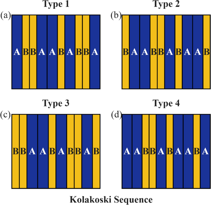
We consider four 1D Kolakoski-type temporal PCs, denoted as Type-I \((\textrm{K}(1,2))\), Type-II \((\overline{\textrm{K}(1,2)})\), Type-III \((\textrm{K}(2,2))\), and Type-IV \((\overline{\textrm{K}(2,2)})\), where Type-II is obtained by swapping Type-I, and Type-IV is obtained by swapping Type-III. Each structure is composed of two temporal media, represented to temporal layers A and B. The sequences are generated through iterative substitution rules, producing deterministic aperiodic arrangements of temporal layers28,29. The Type-I Kolakoski \(\textrm{K}(1,2)\) is a self-generating, quasi-periodic sequence of 1’s and 2’s, defined by its own elements as successive run lengths. It begins as \(\textrm{K}(1,2)=1,2,2,1,1,2,1,2,2,1,2,2,\ldots .\) By assigning \(1\rightarrow \textrm{A}\) and \(2\rightarrow \textrm{B}\), it can be written as \(\textrm{K}(1,2)=\textrm{A,B,B,A,A,B,A,B,B,A,B,B,}\ldots .\). Type-II is obtained by swapping A and B, so \(\overline{\textrm{K}(1,2)}=\textrm{B,A,A,B,B,A,B,A,A,B,A,A,}\ldots \). Type-III is \(\textrm{K}(2,2)=\textrm{B,B,A,A,B,A,B,B,A,B,B,A,A,}\ldots \), and Type-IV is obtained by swapping A and B in Type-III, so \(\overline{\textrm{K}(2,2)}=\textrm{A,A,B,B,A,B,A,A,B,A,A,B,B,}\ldots \). For a sequence \(\textrm{K}(p,q)_{n}\), the subscript n denotes a finite Kolakoski sequence containing n terms/elements. For example, \(\textrm{K}(1,2)_{10}=\textrm{A,B,B,A,A,B,A,B,B,A}\), which is shown as a schematic representation in Fig. 1a. The other sequences, \(\overline{\textrm{K}(1,2)}_{10}\), \(\textrm{K}(2,2)_{10}\), and \(\overline{\textrm{K}(2,2)}_{10}\), are shown in Fig. 1b–d, respectively.
Fig. 1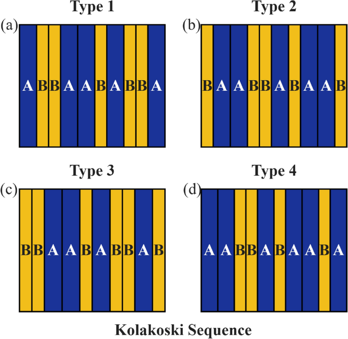
Schematic representation of 1D temporal PCs based on the Kolakoski sequence for different types: (a) Type 1, (b) Type 2, (c) Type 3, and Type 4.
The n determines the total number of temporal layers and, consequently, the structural complexity of the temporal PC. Throughout this work, the relative permittivities of the two temporal media are chosen as \(\varepsilon _{\textrm{A}}=3,\) and \(\varepsilon _{\textrm{B}}=1\), while the relative permeabilities are fixed at \(\mu _{\textrm{A}}=\mu _{\textrm{B}}=1\)20. The refractive indices of the temporal media are given by \(n_{\textrm{A}}=\sqrt{\varepsilon _{\textrm{A}}\mu _{\textrm{A}}}\), and \(n_{\textrm{B}}=\sqrt{\varepsilon _{\textrm{B}}\mu _{\textrm{B}}}\), and the corresponding wave impedances are \(\eta _{\textrm{A}}=\sqrt{\frac{\mu _{\textrm{A}}}{\varepsilon _{\textrm{A}}}}\), \(\eta _{\textrm{B}}=\sqrt{\frac{\mu _{\textrm{B}}}{\varepsilon _{\textrm{B}}}}\)10,11. The temporal durations of the layers, \(t_{\textrm{A}}\) and \(t_{\textrm{B}}\), are defined as the quarter wave condition relative to the time period \(T_0 = 2 \times 10^{-15}\text { s}\) and are defined as
$$\begin{aligned} t_{\textrm{A}} = \frac{T_0\operatorname {Re}\{n_{\textrm{A}}\}}{4} \qquad t_{\textrm{B}} = \frac{T_0\operatorname {Re}\{n_{\textrm{B}}\}}{4} \end{aligned}$$
(1)
where \(\operatorname {Re}\{n_{\textrm{A}}\}\) and \(\operatorname {Re}\{n_{\textrm{B}}\}\) denote the real parts of the respective refractive indices.
The characteristics matrix of the \(j^{\text {th}}\) temporal segment is expressed as30
$$\begin{aligned} S_{j} = \begin{bmatrix} \cos (\omega _{j} t_{j}) & -\dfrac{i}{\eta _{j}} \sin (\omega _{j} t_{j}) \\ -i \eta _{j} \sin (\omega _{j} t_{j}) & \cos (\omega _{j} t_{j}) \end{bmatrix}, \end{aligned}$$
(2)
Here, \(\omega _{j}=kc/n_{j}\) is the frequency of the \(j^{\text {th}}\) segment, and \(t_{j}\) is the temporal duration of the \(j^{\text {th}}\) segment.
The total transfer matrix of the proposed structure is expressed as
$$\begin{aligned} S=\prod _{j=1}^{N}S_{j}=\begin{bmatrix} S_{11} & S_{12}\\ S_{21} & S_{22} \end{bmatrix} \end{aligned}$$
(3)
The transmission of the proposed system is defined by30
$$\begin{aligned} \begin{aligned} T = \left| \frac{ \left( S_{21}-S_{22}\eta _{\textrm{out}}\right) – \left( S_{11}-S_{12}\eta _{\textrm{out}}\right) \eta _{\textrm{in}} }{ \begin{aligned}&\left( S_{11}+S_{12}\eta _{\textrm{out}}\right) \left( S_{21}-S_{22}\eta _{\textrm{out}}\right) \\&-\left( S_{11}-S_{12}\eta _{\textrm{out}}\right) \left( S_{21}+S_{22}\eta _{\textrm{out}}\right) \end{aligned} } \right| . \end{aligned} \end{aligned}$$
(4)
where \(\eta _{\textrm{in}}=\eta _{\textrm{out}}=1\).
Fig. 2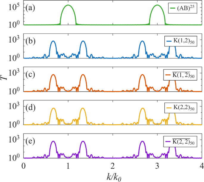
Transmission characteristics of temporal PCs, (a) periodic; based on the Kolakoski sequence for different types: (b) \(\textrm{K}(1,2)_{50}\), (c) \(\overline{\textrm{K}(1,2)}_{50}\), (d) \(\textrm{K}(2,2)_{50}\), and (e) \(\overline{\textrm{K}(2,2)}_{50}\).