Fire risk to U.S. structures nearly triples by mid-century

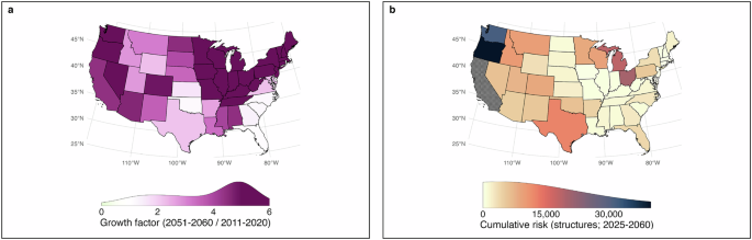
In this study, we estimate spatial and temporal trends in fire risk to structures across the contiguous United States (CONUS). Fire risk is defined following the Intergovernmental Panel on Climate Change (IPCC) framework as the expected loss arising from the interaction between fire hazard, exposure, and vulnerability65. To operationalize this definition, we first estimated spatiotemporal trends in fire hazard by analyzing historical and projected burned area across ecoregions. Second, we quantified changes in development patterns to characterize exposure, measured as the number of structures present across landscapes through time. Third, we refined the conventional fire-risk formulation by incorporating an empirical measure of structural vulnerability that accounts for heterogeneity in fire characteristics and settlement patterns. Finally, we examined projected fire risk under the lens of social vulnerability to assess how biophysical hazard and structural exposure and vulnerability intersect with socioeconomic conditions across communities. All analyses and figures were produced with R 4.3.166, using the packages biscale 1.0.067, classInt 0.4-968, clipr 0.8.069, cowplot 1.1.170, doParallel 1.0.1671, exactextractr 0.9.172, fasterize 1.0.473, foreach 1.5.174, ggpattern 1.1.475, ggplot2 3.5.176, ggpubr 0.6.077, ggtext 0.1.278, ggthemes 4.2.479, Hmisc 5.1-180, mgcv 1.9-181, modEvA 3.1782, pacman 0.5.183, png 0.1-884, pryr 0.1.685, purrr 1.0.286, ragg 1.3.287, raster 3.6-2388, scales 1.3.089, scico 1.5.090, sf 1.0-14, stringr 1.5.091, terra 1.7-3992, tidyverse 2.0.093, viridis 0.6.494, and their corresponding dependencies.

Spatiotemporal trends in fire hazard

We employed data on area burned from the Monitoring Trends in Burn Severity44 and Stephen et al.’s model19 to document (1985-2023) and project (2023-2060) temporal trends in area burned at the EPA Level IV ecoregion scale. The modeling framework, initially developed by Joseph et al.18, integrates a 30-year fire record with meteorological/climatological and population data to construct spatiotemporal models incorporating spatially varying nonlinear effects using Bayesian finite maxima. Model training utilized data from 1984 to 2009, withholding data from 2010 to 2016 for validation. A Hamiltonian Monte Carlo method, implemented in the probabilistic programming language Stan, was used for parameter estimation. Four chains of 1000 iterations each were executed, with the first 500 iterations discarded as a warm-up phase. For this study, we derived weather/climate ensemble results from three General Circulation Models (GCMs) under the RCP 4.5 emissions scenario, namely, Centre Régional de Recherches Météorologiques Model (CNRM), Hadley Centre Global Environmental Model—Earth System version (HadGEM-ES), and Meteorological Research Institute Model (MRI).

Characterization of the built environment

Changes in settlement patterns are typically mapped using satellite imagery or other spatial data offering insights into land use and the built environment95,96. However, these data sources present certain spatial and temporal characteristics that constrain their effectiveness in risk assessments. Extensive, high-resolution remotely sensed data, for example, have only been available since the advent of satellite technology in the 1970s, precluding long-term historical analyses. Additionally, these data sets often employ coarse classifications of development intensity and offer less reliability in rural regions42. The limitations of remotely-sensed products in settlement analysis include resolution constraints, spectral and temporal limitations, data integration challenges, misclassification issues, and reliance on ancillary data for validation97.

To overcome these limitations, we relied on property-record data representing the historical built environment. Specifically, we employed the Historical Settlement Data Compilation for the US (HISDAC-US26,42,43). HISDAC-US provides a gridded time series of settlement layers derived from the Zillow Transaction and Assessment Data set (ZTRAX), which includes over 370 million records on housing and land-parcel attributes.

From this dataset, we extracted Built-Up Property Records (BUPR) gridded surfaces, which contain residential, commercial, industrial, non-profit, and agricultural buildings or building units within 250 × 250 m grid cells across the conterminous United States from 1810 to 2020. BUPR constitutes an empirical record of historical settlement patterns derived from property assessment data. To refine our dataset, we integrated information from the U.S. Geological Survey’s Protected Areas Database (PAD-US 4.0) and excluded structures located on federal, tribal, state, or local public lands. The resulting dataset represents privately owned structures located on private land, including residential properties, as well as commercial and industrial buildings. We focused on privately owned structures for two primary reasons. First, the HISDAC-US database is derived from property assessment records, which are most complete and consistently reported for privately owned parcels, whereas structures on public lands (e.g., administrative facilities, recreation infrastructure, utility buildings) are often inconsistently represented or absent from parcel-based tax assessment systems. Second, the majority of wildfire-related structural losses recorded in national incident reporting datasets (e.g., ICS-209-Plus) occur within privately owned residential and mixed-use developments, which constitute the dominant component of the built environment at risk from wildland–urban interface fires. This approach may omit a small number of publicly owned structures affected by wildfire (e.g., National and State Park facilities), but these structures represent a minor fraction of the national structure inventory and do not substantially influence large-scale estimates of wildfire risk to the built environment.

Settlement patterns were analyzed by overlaying these layers with EPA Level IV ecoregions across the CONUS. For each ecoregion s and year t, the number (Eq. 1) and density of structures (Eq. 2) was calculated as:

$$N(s,t)={\sum}_{g\in s}{n}\left({\mbox{g}},{\mbox{t}}\right)$$

(1)

$$D(s,t)=N(s,t)/A(s)$$

(2)

where N(s,t) is the total number of structures in ecoregion s at time t, n(g,t) denotes the number of structure records in grid cell g located within ecoregion s at time t, D(s,t) is structure density, and A(s) is the area of ecoregion s.

Estimation of temporal trends in development

Temporal trends in the number of structures per EPA Level IV Ecoregion between 1940 and 2060 were estimated with Generalized Additive Models (GAMs), which allow non-linear relationships between predictors and response variables through smooth functions98,99. We iteratively fitted both Negative Binomial and Poisson GAMs to the number of structures in each ecoregion as a function of time.

The Negative Binomial model is expressed as (Eq. 3):

$$N(t) \sim {{{\rm{NB}}}}(\mu (t),\,\theta )$$

(3)

where NB(μ(t), θ) represents a Negative Binomial distribution with mean μ(t) and dispersion parameter θ.

The expected value μ(t) is modeled as (Eq. 4):

$$\log \mu (t)={{{\rm{\beta }}}}0+f(t)$$

(4)

where \(\beta\)0 is the intercept and f(t) is a smooth function of time (thin-plate regression spline).

The smoothing function is estimated using a penalized cubic regression spline (Eq. 5):

$$f(t)={\sum}_{k=1}^{K}{\beta }_{{{{\rm{k}}}}}{{\mbox{B}}}_{{{{\rm{k}}}}}({\mbox{t}})$$

(5)

where Bk (t) are spline basis functions, and βk are the corresponding spline coefficients estimated using Restricted Maximum Likelihood (REML).

To ensure appropriate distributional assumptions, we also used Poisson GAMs to model the number of structures per Level IV ecoregion as a function of year (Eq. 6):

$${{{\rm{N}}}}(t) \sim {{{\rm{Poisson}}}}(\lambda (t))$$

(6)

where Poisson (λ(t)) represents a Poisson distribution with mean λ(t) and dispersion parameter λ. The log-link function (Eq. 7) was then applied so that:

$$\log \lambda (t)={\beta }_{0}+f(t)$$

(7)

where β0 is the intercept and f(t) is the smoothing function defined above (Eq. 5).

For each ecoregion s, we calculated the Akaike Information Criterion (AIC100) (Eq. 8):

$${{{\rm{AIC}}}}=2m-2\log L$$

(8)

where m is the number of estimated parameters and L is the model likelihood. AIC is a widely used metric for model selection that balances goodness of fit with model complexity, penalizing overfitting. By choosing the model with the lowest AIC, we ensured that the selected model provided the best compromise between explanatory power and generalizability.

Model validation

To ensure model robustness, we validated the GAMs by comparing the predicted number of structures per Level IV ecoregion to an independent 30% holdout set excluded from training. Model performance was evaluated based on the percentage of deviance explained between observed and predicted values. This approach enabled us to test the models’ ability to capture temporal trends in settlement patterns across diverse ecological regions.

Comparison with population data

Given that population growth is the primary driver of housing demand, we used population estimates as a real-world benchmark to assess whether our built-environment estimates aligned with reasonable expectations. To this end, we obtained population estimates from the Integrated Climate and Land Use Scenarios Version 2 (ICLUS v235). These projections are based on demographic models incorporating fertility, mortality, and migration rates, and integrate Representative Concentration Pathways101. In the context of population projections, ICLUS provides detailed data sets consistent with the Shared Socioeconomic Pathways (SSPs) narratives. For example, under SSP2, which represents a “middle-of-the-road” scenario, the U.S. population is projected to reach ~455 million by 2100. In contrast, SSP5 describes a rapidly growing global economy heavily reliant on fossil fuels, leading to a U.S. population exceeding 730 million by 2100.

Under the assumption that increases in population lead to the construction of new housing units to maintain stable occupancy levels, we computed temporal trends in occupancy as the ratio of population to the number of structures per Level IV ecoregion as (Eq. 9):

$$O(s,t,{spp})=P(s,t,{spp})/N(s,t)$$

(9)

where O(s, t, spp) is the occupancy in ecoregion s in year t under shared socioeconomic pathway ssp, P(s, t, spp) is the projected population of ecoregion s in year t under shared socioeconomic pathway ssp, and N(s, t) is the corresponding estimated number of structures.

Additionally, we calculated cross-correlation functions (CCF) between the modeled number of structures and different SSP-based population estimates at 10-year lags.

Fire risk to the built environment

The conventional risk formulation (Eq. 10) assumes that risk, or structural loss, is determined by hazard and exposure102:

$$R({s}_{3},t)={p}_{f}({s}_{3},t)N({s}_{3},t)$$

(10)

where the fire risk to structures in ecoregion s3 and year t, R(s3, t), is a function of the probability of fire pf (s3, t) and the number of structures, N(s3, t), in Level III ecoregion s3 and year t.

Because this formulation assumes uniform fire characteristics and equal vulnerability across structures, it does not capture the substantial heterogeneity in structural loss observed across regions. To address this limitation and provide a more realistic representation of fire risk to structures, we estimated an empirical term, which approximates structure loss conditional on structure density and burned area within each ecoregion. This quantity, referred to as the Exposure-Adjusted Structure Loss Index (EASLI), is defined as (Eq. 11):

$${p}_{d}\left({s}_{3}\right)=D({s}_{3})/(N({s}_{3}){p}_{a}({s}_{3}))$$

(11)

where pd (s3) is the annual probability of damaging or destroying a structure given that a fire occurs in ecoregion s3, D(s3) represents the annual number of structures damaged or destroyed by fire in ecoregion s3, N(s3) is the total number of structures in ecoregion s3, and pa(s3) is the proportion of ecoregion s3 burned annually.

Structural loss observations D(s3) were obtained from the ICS-209-Plus dataset (2000–202333). Structure inventories N(s3) were derived from BUPR settlement data, and burned area B(s3) was calculated from MTBS fire perimeter records37.

The annual burned-area proportion was calculated as (Eq. 12):

$$pa({s}_{3})={{{\rm{B}}}}({s}_{3})/{{{\rm{A}}}}({s}_{3})$$

(12)

where the mean annual area burned, B(s3), was derived from MTBS fire perimeters aggregated at the Level III ecoregion, and A(s3) is the area of ecoregion s3.

By incorporating spatially explicit fire occurrence and structural loss data, EASLI provides a more realistic estimate of structural susceptibility to fire. This index can be interpreted as an approximation to the annual probability that any given house in a given ecoregion will be affected by fire conditional on the number of structures and the area burned.

Integrating hazard, exposure, and structural vulnerability yields the final risk formulation (Eq. 13):

$$R(s,t)=pa(s,t)N(s,t)pd({s}_{3})$$

(13)

In this formulation, hazard corresponds to the proportion of area burned, exposure corresponds to the number of structures present, and structural vulnerability corresponds to the empirically derived EASLI metric. Their product yields the expected number of structures damaged or destroyed by wildfire.

Sensitivity analysis of the exposure-adjusted structure loss index and risk components

To evaluate the robustness of the Exposure-Adjusted Structure Loss Index (EASLI) and to quantify the relative contributions of hazard, exposure, and structural vulnerability to fire risk, we implemented a multi-step sensitivity and decomposition framework combining bootstrap uncertainty analysis with variance and temporal decomposition methods.

Bootstrap-based uncertainty in EASLI

The sensitivity of in EASLI to sampling variability in the historical record was quantified using nonparametric bootstrap resampling103. Annual observations of burned-area proportion, structure counts, and observed structural losses were resampled with replacement (B = 2000) within each EPA Level III ecoregion. For each bootstrap replicate, EASLI was recomputed, preserving the joint dependence structure among hazard, exposure, and loss. For each ecoregion, the bootstrap distribution of EASLI pd was summarized using the mean, median, standard deviation, and percentile-based 95% confidence intervals. Multiplicative uncertainty was characterized using the geometric standard deviation in log space, reflective of the strictly positive, right-skewed ratios commonly encountered in the analysis.

Bootstrap realizations were additionally used to evaluate the robustness of regional differences in EASLI and the stability of inferred risk patterns. For each replicate, ecoregions were ranked according to estimated risk while holding hazard and exposure constant, such that variation in rank reflects uncertainty in EASLI alone. The resulting rank distributions were used to estimate the probability that a given ecoregion consistently falls within the highest 20%, middle 60%, or lowest 20% of risk values. These probabilities quantify the confidence with which ecoregions can be assigned to relative vulnerability tiers, distinguishing regions with persistently high or low exposure-adjusted losses from those whose rankings are sensitive to sampling variability.

Observed structural losses from the ICS-209-Plus dataset were used as an independent benchmark to assess whether ecoregions identified as high-vulnerability under the model correspond to historically high-damage regions. This comparison informs the empirical validity of the EASLI metric as a proxy for realized structural loss patterns.

Spatial attribution of risk components

To evaluate the influence of EASLI on structure loss risk, we decomposed risk into its constituent components: number of structures, proportion of area burned, and EASLI across EPA Level IV Ecoregions. Given the multiplicative nature of risk [Eq. 13], we expressed this relationship in log space (Eq. 14):

$$\log (R(s,t))=\log ({p}_{a}(s,t))+\log (N(s,t))+\log (pd({s}_{3}))$$

(14)

We then quantified the relative influence of EASLI by computing the magnitude of each component’s contribution to total log-risk using an absolute-share decomposition104 (Eq. 15):

$$ {Ci}(s)=|\!\log (X_{i}(s))|/(|\!\log (p_{\!a}(s))|+|\log (N(s))|+|\log (p_{d}(s))|),\\ {{{\rm{where}}}}\,{X}_{i}(s)\in \{{p}_{a}(s),N(s),{p}_{d}(s)\}$$

(15)

This yields three normalized contributions C, i.e., share of structures, share of area burned, and share of EASLI, that sum to 1 for each ecoregion s. Each share represents the relative magnitude of that component’s contribution to the total log-scale risk signal. Using absolute values ensures that contributions reflect magnitude rather than direction, which is necessary because log-transformed components may differ in sign depending on their scale relative to unity. This formulation enables direct comparison of the influence of EASLI against exposure and fire activity across heterogeneous ecoregions.

Temporal attribution of risk change

Building on the same log-space decomposition approach (Eq. 14), we calculated the relative contribution of each risk component to temporal changes in structure loss risk. Annual observations were first aggregated into consecutive 5-year periods beginning in 2000. We then quantified inter-period variability by calculating first differences in log-risk and its components between consecutive 5-year periods. The relative contribution of each component to total change was defined using an absolute-change share (Eq. 16):

$$ {{{AC}}_{i}}^{\Delta }=|\Delta \log ({X}_{i}(s))|/(|\Delta \log ({p}_{a}(s))|+|\Delta \log (N(s))|+|\Delta \log ({p}_{d}(s))|),\\ {{{\rm{where}}}}\,{X}_{i}(s)\in \{{p}_{a}(s),N(s),{p}_{d}(s)\}$$

(16)

The decomposition produces three normalized contributions AC, share of area burned, share of number of structures, and share of EASLI, that sum to 1 for each transition between consecutive 5-year periods. Each share represents the magnitude of that component’s contribution to the total change in log-risk.

Socioeconomic vulnerability and fire risk

We used version 2 of the Climate and Economic Justice Screening Tool105 to obtain socioeconomic data, focusing on the percentage of households below 200% of the federal poverty line and housing cost burden across all census tracts in the CONUS. For each tract, we estimated both current and future fire risk by calculating the area-weighted mean fire risk, using the overlap between EPA Level IV ecoregions and census tracts as weights. Each variable was categorized into three classes, resulting in two distinct 3 × 3 bivariate classification schemes: fire risk vs. poverty, fire risk vs. housing burden. These relationships were visualized using bivariate choropleth maps to illustrate spatial patterns of overlapping social vulnerability and fire risk to structures.

Reporting summary

Further information on research design is available in the Nature Portfolio Reporting Summary linked to this article.