Multiancestry brain pQTL fine-mapping and integration with genome-wide association studies of 21 neurologic and psychiatric conditions

Ethics

Our study complies with all relevant ethical regulations and was approved by the institutional review boards at University of California, Davis; Rush University; the Mayo Clinic; Mount Sinai University; Emory University and Banner Sun Health Research Institute.

Genetic data

Genetic data were generated from blood or brain tissue using either array-based genotyping or whole-genome sequencing (WGS) as described previously19,20,21,22. New to this study was WGS from 181 AA, 168 Hispanic and 292 NHW individuals whose raw Illumina 150-bp reads were mapped to GRCh38 to a median depth of 30× with PEMapper23. Genetic variants were jointly called across samples with PECaller (v.2.0.1)23 using default parameters.

Quality control of genetic data

We prioritized use of WGS over genotyping where available and performed quality control of WGS and genotyping data separately using PLINK24. Participants with overall genotyping missingness >10% and sex mismatch were excluded. Variants with evidence of deviation from Hardy–Weinberg equilibrium (P < 10−7) and missing genotype rate >5% were removed. Genotype data in GRCh37 were converted to GRCh38. We followed the quality-control steps provided by the TOPMed pipeline25 for genetic data before imputation. Imputation was performed using the TOPMed imputation panel and server with default parameters25. SNPs with imputation quality R2 > 0.3 were retained.

For WGS, we assessed the coverage, missingness, ratio between the number of transition mutations and the number of transversion mutations, and the silent/replacement ratio (the ratio between synonymous and nonsynonymous mutations). We merged the imputed genotyping data and WGS data and performed further quality control in each population (AA, Hispanic and NHW) separately by excluding variants with any of the following criteria: genotype missing rate >5%, MAF < 5%, nonbiallelic variants and Hardy–Weinberg equilibrium P < 10−7.

Related individuals were identified using KING (v.2.2.2)26, and one in each pair of individuals who were second-degree or closer relatives was randomly removed. Individuals who were population outliers were identified and removed using EIGENSTRAT from EIGENSOFT (v.8.0.0)27.

Benchmarking ancestry and/or ethnicity

All participants with individual-level genetic data were divided into three populations based on self-report: AA, Hispanic and NHW. Within each self-report population, we removed outliers based on genetic ancestry by performing multidimensional scaling analysis using individual-level genetic data and phase 3 1000 Genomes data as in ref. 28. Self-defined Hispanic study participants were combined with the MXL (Mexican ancestry in Los Angeles, CA), PUR (Puerto Rican), CLM (Columbian) and PEL (Peruvian) reference panel populations. Self-defined NHW study participants were combined with the CEU (Utah residents with northern and western European ancestry), TSI (Toscani in Italy), IBS (Iberian population in Spain) and FIN (Finnish) reference panel populations. Self-reported AA participants were combined with the ASW (African ancestry in southwest USA) population. Within each of the three populations, SNPs were filtered to meet the criteria MAF > 5%, data missingness <0.1 and Hardy–Weinberg equilibrium P < 10−7 using an independent pairwise linkage filter window of 50 kb at 5 kb steps and an r2 threshold of 0.15. We removed AT, TA, GC and CG markers. Then, for each group, multidimensional scaling analysis was performed using PLINK (v.1.90b53)24, and results were visualized along principal components 1 and 2 using R. For each population, samples that were six or more standard deviations from the mean of any reference panel populations were considered outliers and removed (42 in the NHW population, 4 in the AA population and 4 in the Hispanic population).

LD panel for each population for PWASs and PMR-Egger

We generated an LD panel for integration of GWASs and brain proteomic and genetic data for each population separately. For NHW, we used the LD reference panel from the 1000 Genomes European data provided in the FUSION pipeline3. For African ancestry, we constructed an LD panel using the AFR HapMap SNP sites in the AFR 1000 Genome data28. Likewise, for the Hispanic population, we constructed an LD panel using the AMR HapMap SNPs in the AMR 1000 Genome data28.

Proteomic dataProteomic sequencing and database search

Proteomic data were generated by collaborative efforts of the Accelerating Medicines Partnership: Alzheimer’s Disease (AMP-AD)29 and AMP-AD Diversity22,30 involving multiple research sites. Brain samples were collected by Rush Alzheimer’s Disease Center (n = 815), the Mayo Clinic (n = 399), Mount Sinai University Hospital (n = 205), Emory University (n = 129) and the Brain and Body Donation Program at Banner Sun Health (n = 200) for proteomic studies as previously reported7,21,22,30. All donors or their next of kin provided informed consent, and the study was approved by the respective institutional review boards at all sites. AMP-AD generated data from samples collected by Rush and Banner Sun Health. AMP-AD-Diversity generated data from samples provided by Rush, the Mayo Clinic, Mount Sinai and Emory. Proteomes were profiled using tandem mass tag mass spectrometry as described in detail previously21,30. Briefly, postmortem brain samples were homogenized, and proteins were digested with trypsin. Samples were randomized for sex, age, diagnosis, and race and/or ethnicity and labeled with isobaric tandem mass tag peptides. All proteomic sequencing batches included at least one global internal standard (GIS). The GIS were created by aliquoting equal amounts of protein from each sample within a batch; these standards were then digested in parallel with other samples within the batch31. Next, high-pH fractionation was performed, and the resulting samples were analyzed by liquid chromatography coupled to tandem mass spectrometry. Raw files were searched using Fragpipe (v.19.0)32, MSFragger32 (v.3.5) and human proteome database Swiss-Prot33 containing 20,402 sequences (downloaded 11 February 2019). Subsequently, we used Post-MSFragger (v.3.6) and Percolator34 (v.3.0.5) for peptide–spectrum match validation and Philosopher (v.4.6.0) for protein inference using ProteinProphet (v.4.6.0) and filtering using FDR. The database search yielded a total of 11,748 protein groups from the dorsolateral prefrontal cortex.

Quality control and normalization of proteomic data

We examined proteomic assay precision via coefficient of variation (CV) analysis, using the 7 batches with ≥2 GIS (a total of 15 within-batch GIS). Lower CVs reflect lower measurement errors and higher precision. Based on protein abundance before normalization, we calculated the CV for each gene within each batch using the formula CV = s.d.(x)/mean(x), where x is the protein abundance for each gene in the GIS samples within each batch. We found the CVs to have a median of 2.2, interquartile range of 1.8 and range of [0.23–23.1] among 7,675 proteins without any missing values, suggesting very high reproducibility. We performed quality control of proteomic data in the AMP-AD-Rush (n = 619), AMP-AD-Banner (n = 198) and AMP-AD-Diversity (n = 1,105; Rush, Mayo, Mount Sinai, Emory; Supplementary Table 25) datasets separately following our prior approach7,21,35,36. Specifically, in each of the three datasets, we performed the following steps. First, we removed duplicate samples (only AMP-AD-Diversity had duplicate samples, and one of the pair was removed). Second, we removed proteins with missing values in more than 50% of the samples. Third, the protein abundance for each gene per sample was normalized using the total abundance of all the proteins in that sample to account for protein loading differences and then log2-transformed. Fourth, we performed iterative principal component analysis to remove sample outliers that were more than four standard deviations from the mean of either the first or the second principal component. Fifth, we performed linear regression to estimate and remove the effects of protein sequencing batch, PMI, age at death, sex and clinical diagnosis of cognitive status from the proteomic profiles. In the AMP-AD-Diversity dataset, a subset of the samples did not have PMI (n = 149). Thus, we performed regression to remove unwanted technical and biological effects in the subset with PMI separately from the subset without PMI. Last, to enable comparisons across the three datasets (AMP-AD-Rush, AMP-AD-Banner and AMP-AD-Diversity), a Z-score transformation of the protein abundance for each protein to a mean of 0 and standard deviation of 1 was applied within each dataset. For proteins with multiple isoforms, we selected the most abundant isoform for investigation. Variance partition plots showing the contributions of technical and biological effects to the proteomic profiles before and after quality control and normalization for these three datasets are provided in Supplementary Figs. 1–3.

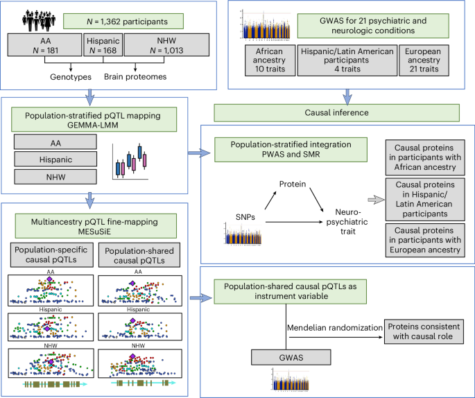
Next, we combined the proteomic profiles from the three datasets and retained samples having both proteomic and genetic data. Then we performed additional quality control of the proteomic data in each population (AA, Hispanic and NHW) separately as follows. First, we retained proteins with nonmissing data in at least 50 individuals. Second, we performed surrogate variable analysis (SVA v.3.20.0)37 on the proteomic profile to assess potentially hidden confounding variables and regressed out the significant surrogate variables from the normalized proteomic profile. Last, Z-score transformation of the surrogate-variable-adjusted protein abundance for each protein was applied to the proteomic profile in each population. After quality control of genetic and proteomic data as described above, a total of 1,362 individuals remained for pQTL mapping. They comprised 181 AA (9,304 proteins), 168 Hispanic (9,036 proteins) and 1,013 NHW (9,725 proteins) individuals (Supplementary Table 24).

Population-stratified pQTL mapping

pQTL mapping in each population was performed for SNPs present at MAF ≥ 0.05 in a population. We defined cis as being within 500 kb up or downstream of the gene. We fitted an LMM with SNP as the independent variable and normalized protein expression as the outcome, adjusting for sex using GEMMA (v.0.98.1)4. We chose an LMM as it could account for sample relatedness and population substructure. We calculated the P value using the Wald test in GEMMA. As described above, we regressed our the surrogate variables from the proteomic profile of each population before performing pQTL mapping. The genomic inflation factor (λ) was calculated by dividing the median of the resulting chi-squared test statistics by the expected median of the chi-squared distribution38.

Influence of allele frequency differences on population-specific pQTLs

We investigated whether differences in pQTL detection were related to differences in allele frequencies between populations. Here we defined AA-only candidate pQTLs as those identified as pQTLs in AA that were not pQTLs in NHW and were found to have ≤1 minor allele in European populations in the 1000 Genomes WGS data. Among the 144,654 candidate pQTLs in AA from the population-stratified pQTL mapping, we found 14,239 AA-only candidate pQTLs, corresponding to 1,578 independent AA-only candidate pQTLs (after clumping at r2 < 0.1) and constituting 12.8% of the 7,852 independent candidate pQTLs identified in the AA population. Likewise, we defined NHW-only pQTLs as those that were candidate pQTLs in NHW but not in AA and had ≤1 minor allele in African populations in the 1000 Genomes data. Among the 1,328,595 candidate pQTLs in NHW from the population-stratified pQTL mapping, we found 3,939 NHW-only candidate pQTLs, which corresponded to 1,271 independent NHW-only candidate pQTLs (after clumping at r2 < 0.1) and constituted 1.1% of the 40,087 independent candidate pQTLs identified in the NHW population.

Fine-mapping

Multiancestry pQTL fine-mapping was performed with MESuSiE (v.1.0)8, which considers only proteins and SNPs that are present in all examined populations. We considered SNPs present at MAF > 0.05 in each population. Inputs to MESuSiE included the summary statistics of the population-stratified pQTL mapping and LD matrix for each population. The LD matrix for each population was generated using the same individual-level genotyping and/or WGS data used in the population-stratified pQTL mapping to ensure there was no mismatch between the population-stratified pQTL summary statistics and the LD matrix. We performed an LD mismatch check following MESuSiE guidelines. We set the L parameter (that is, the maximum number of possible credible sets) to the default value of 10. As we performed multiancestry pQTL fine-mapping in three populations, there were seven possible pQTL categories: (1) shared across AA, Hispanic and NHW; (2) shared between AA and Hispanic; (3) shared between AA and NHW; (4) shared between Hispanic and NHW; (5) specific to AA; (6) specific to Hispanic; and (7) specific to NHW. The output from MESuSiE included the PIP for each of these categories, referred to as the category.PIP. We then applied additional filters to the MESuSiE results to remove causal pQTLs with category assignments discordant with the population-specific pQTL results. Specifically, among causal pQTLs categorized as shared across populations, we filtered out those that were not nominally significant in each population (that is, P > 0.05) or had discordant beta values. Likewise, for the causal pQTLs categorized as population-specific, we filtered out those that had population-stratified pQTL P < 0.05 in other populations.

pQTL fine-mapping in NHW with SuSiE

To compare the size of the 95% credible sets between multiancestry pQTL fine-mapping and NHW-only pQTL fine-mapping, we performed pQTL fine-mapping in NHW with susieR (v.0.12.35)9 following its default pipeline. SuSiE was designed to identify as many credible sets as the data would support, each with as few variants as possible. For a given gene and its corresponding variants in the cis-regulatory region, the output was the number of credible sets that had 95% probability of containing a variant with nonzero causal effect. We set the maximum number of credible sets for a gene to be ten (the default value).

Influence of sample size on population-shared and -specific pQTLs

We downsampled the NHW proteomic dataset from 1,013 to 191 to make it comparable to the sample sizes for the AA and Hispanic populations. The smaller NHW group (EUR-2) had similar distributions of age, sex and PMI as the larger NHW group. We performed population-stratified pQTL mapping for each group (EUR-2 n = 191; AA n = 181; Hispanic n = 168) and used the pQTL summary statistics as an input for multiancestry pQTL fine-mapping with MESuSiE.

Genomic-site-type enrichment

Genomic-site-type annotations for the 3,643,245 SNPs tested in all three populations in the population-stratified pQTL analyses were obtained using Bystro (v.2.0.0-beta1)39. SNPs were annotated with the following site types: nonsynonymous, synonymous, UTR or intronic. In each case, the annotation was assigned to a SNP if and only if it pertained to one or more of the genes tested for the SNP. Promoter overlap for each SNP was determined using the promoter-like candidate cis-regulatory elements from ENCODE40. Fisher’s exact test was used to test enrichment of each site type in two sets of pQTLs: the multiancestry causal pQTLs from MESuSiE and the shared candidate pQTLs from the population-stratified pQTL analyses. As the shared candidate pQTLs included many SNPs in LD, a set of approximately independent SNPs was selected by applying the –clump function from PLINK to greedily select pQTLs with pairwise LD < 0.1. For both sets, a SNP was counted as ‘in the set’ if it was a pQTL for any gene.

Cross-ancestry prediction of genetically regulated protein abundance

Focusing on the 858 multi-ancestry causal pQTLs, we included SNPs in their corresponding 95% credible sets. Then, we computed the effect of these SNPs on protein abundance (also referred to as protein ‘weights’) using NHW genetic and proteomic data and multiple predictive models (top1, blup, lasso, enet and bslmm) following the FUSION framework3. We extracted the protein weights from the most predictive models. Next, we estimated the genetically regulated protein abundance for the pGenes corresponding to the multiancestry causal pQTLs using AA genotyping and the above protein weights. Subsequently, we calculated the R2 and P value for regression of the predicted AA proteomic expression on the measured AA proteomic expression to provide estimates of cross-ancestry prediction accuracy.

In addition, we performed same-ancestry prediction following the pipeline described above using AA genetic and proteomic data for the pGenes corresponding to the 858 multiancestry causal pQTLs. Following the FUSION framework, we used all the SNPs corresponding to the pGenes for the 858 multiancestry causal pQTLs. The output provided cross-validation R2 values for the best-performing models. The R2 metric reflects the percentage variance of protein abundance explained by the genetically regulated protein level, with higher values corresponding to more variance explained. To compare the cross-ancestry to the same-ancestry prediction, we took the ratio of the cross-ancestry and same-ancestry cross-validation R2 values.

π
1 replication rate for pQTLs

To determine the π1 rate for the multiancestry causal pQTLs in each of the populations, we first estimated π0, which is the proportion of true null hypotheses among a set of tests, using R package qvalue (v.2.15.0). In the case of our application to P values from the LMM tests, the null hypothesis was that the SNP had zero effect on protein expression. π1, the proportion of true alternative hypotheses, was defined as 1 − \({\pi }_{0}\).

To compare the pQTLs and pGenes identified here in the NHW population with those from our previous published brain pQTL study using a smaller dorsolateral prefrontal cortex dataset7, we extracted significant pQTLs and pGenes from each study (FDR < 0.05) and identified overlapping and unique findings. To estimate π1 rates using the current brain pQTLs as the discovery set and published plasma pQTLs as replication sets, we extracted the population-stratified brain pQTLs (at FDR < 0.05) in the current study and examined them in each of the published plasma datasets to estimate π0. In addition, we estimated π1 for the multiancestry causal pQTLs (n = 858) in each of the two plasma pQTL datasets in African and European ancestry populations separately following a similar procedure.

To determine which pGenes were shared between brain and plasma, we focused on European ancestry owing to the higher sample sizes and statistical power. We defined pGenes as proteins with cis-pQTLs at FDR < 5%. To make the plasma pGene definition comparable to our current brain pGene definition, for each protein, we considered SNPs within 500 kb of the gene and estimated the FDR using published plasma pQTL summary statistics in each of the European plasma datasets (Icelanders41, ARIC5 and UKB6). For each comparison, we considered only genes available in both brain and plasma datasets. We examined the overlap between brain and plasma pGenes (‘shared’ pGenes) and the pGenes found only in brain analysis or plasma analysis (‘unique’ pGenes) for each plasma pQTL dataset (Supplementary Tables 25–27). Of our brain pGenes, we found that 91% shared pGenes with plasma pGenes from the Icelanders dataset, 84% shared pGenes with ARIC plasma pGenes and 98% shared pGenes with UKB plasma pGenes (Supplementary Table 28).

GWAS summary statistics

We had access to GWAS summary statistics for 15 psychiatric traits: alcohol use disorder42, anorexia nervosa43, anxiety44, ADHD45, autism spectrum disorder46, bipolar disorder47, cannabis use disorder48, insomnia49, major depressive disorder50,51, neuroticism52, opioid addiction53, PTSD54, schizophrenia55, suicide attempt56 and tobacco use57. We also had summary statistics for six neurologic traits: Alzheimer’s disease58,59, amyotrophic lateral sclerosis60, frontotemporal dementia61, Lewy body dementia62, Parkinson’s disease63,64 and stroke65. We used these results to integrate brain proteomes with GWASs in PWASs, SMR and PMR-Egger as described below.

Integrating GWASs with brain proteomes using PWASs and SMR

For each of the 21 psychiatric and neurologic conditions, we integrated GWAS summary statistics with brain proteomic and genetic data in each population separately using the population-matching GWAS, brain proteome and LD reference panel. All gene coordinates were based on GRCh38. We performed two independent but complementary integration approaches. First, we performed a PWAS of each trait using FUSION3 (https://github.com/gusevlab/fusion_twas, commit e1ba5f7). We restricted the genotype data to the SNPs in the LD reference panel in each population. SNP-based heritability for each protein was estimated, and proteins with SNP-based heritability P < 0.01 were considered to be heritable. For each heritable protein, we estimated the effect of a set of SNPs within a 500-kb window of the gene on its protein abundance. We applied BLUP, LASSO, elastic net and BSLMM prediction models and kept the weights from the best-performing prediction model. Subsequently, we integrated the brain protein weights with each of the GWAS summary statistics to perform a PWAS for each trait in each population for which GWAS results were available, to identify the cis-regulated proteins associated with the trait. We defined significant proteins as those with FDR < 0.05.

In the second approach, among the significant cis-regulated proteins identified in the PWAS described above, we performed summary data-based Mendelian randomization with SMR10 to test whether the brain protein mediated the association between the SNP and trait. We used the population-stratified pQTLs and GWAS summary statistics for each trait in each population separately. As mediation can arise from causality, pleiotropy or LD, we then used HEIDI10 to test for and remove associations likely to be due to LD (that is, HEIDI P < 0.05). We defined proteins consistent with a causal role as those with PWAS FDR < 0.05, SMR P < 0.05 and HEIDI P > 0.05 and a consistent direction of association between protein and trait in the PWAS and SMR.

PMR-Egger using population-stratified data

As an alternative approach to the above PWAS and SMR framework, we used PMR-Egger as implemented in PMR (https://github.com/yuanzhongshang/PMR, commit 7e49f14) to perform SNP–protein–disease causal inference using pQTL and GWAS summary statistics. PMR-Egger is a probabilistic two-sample Mendelian randomization that also controls for horizontal pleiotropy11. Unlike traditional Mendelian randomization approaches that use independent instruments, PMR uses correlated instruments and has similar detection power to PWAS approaches such as FUSION3. It also accounts for horizontal pleiotropy and provides a P value for the effect of horizontal pleiotropy. We ran PMR with function PMR_summary_Egger for each gene in each population (NHW, AA and Hispanic) with our pQTL data and published GWAS results, the same data used in the PWAS and SMR analyses described above, following the instructions in the developer’s example (https://github.com/yuanzhongshang/PMR/tree/master/example). We ran PMR-Egger only for genes that passed the heritability test in the PWAS analysis and calculated an LD matrix for each population using individual-level genetic data from postmortem brain donors. To account for potential mismatches between GWAS data and the LD matrix, we performed an LD mismatch check per MESuSiE guidelines and removed mismatching SNPs before the PMR-Egger run.

Identifying multiancestry causal pQTLs in psychiatric and neurologic conditions through Mendelian randomization

In each population separately, we modeled the 858 multiancestry causal pQTLs as the instrumental variable in Mendelian randomization analysis with SMR10 using the population-matching GWAS and pQTL summary statistics. We declared multiancestry causal pQTLs to be consistent with a causal role if they had SMR FDR < 0.05 and HEIDI P > 0.05 for the trait of interest.

Physical PPIs

The BioGRID database (v.4.4.232; 28 April 2024)66 was used to obtain pairwise protein interactions containing only human gene symbols, which were further filtered to include only physical PPIs such as physical associations and direct interactions, associations and colocalization.

Gene set enrichment analysis

For causal proteins for each trait, gene set enrichment analysis was performed using GO-Elite (v.1.2.5)67 with the background gene set of 9,725 proteins that remained after comprehensive quality control. Causal proteins were subjected to Fisher’s exact overlap test and Z-test in the Python command-line version of GO-Elite, setting the species as Homo sapiens and using the current annotation databases for gene ontology biological processes, molecular functions, cellular components, Wiki pathways, KEGG, REACTOME and CORUM (downloaded April 2024)68.

Reporting summary

Further information on research design is available in the Nature Portfolio Reporting Summary linked to this article.