
Quantum and classical model
The theory of Talbot–Lau interference is best formulated in phase space using the Wigner–Weyl representation of quantum mechanics42. This framework can account for incoherent particle sources, phase and absorption gratings, and all laser-induced photophysical effects, as well as any relevant decoherence process. It also allows for a direct comparison between the predictions of quantum and classical mechanics within the same formalism and set of assumptions.
For a cluster with mass m and longitudinal velocity vz, the probability of being detected behind the interferometer can be written as a Fourier series in the transverse position x3 of G3:
$$S({x}_{3})=\mathop{\sum }\limits_{{\ell }=-\infty }^{\infty }{S}_{{\ell }}\exp \left({\rm{i}}\frac{2{\rm{\pi }}{\ell }}{d}{x}_{3}\right).$$
(1)
In a symmetric setup with equal grating separations L and periods d, the Fourier coefficients are
$${S}_{{\ell }}={B}_{-{\ell }}^{(1)}(0){B}_{2{\ell }}^{(2)}\left({\ell }\frac{L}{{L}_{{\rm{T}}}}\right){B}_{{\ell }}^{(3)}(0),$$
(2)
where the Talbot–Lau coefficients \({B}_{{\ell }}^{(j)}\) of order ℓ for the jth grating still need to be determined as a function of the Talbot length LT = mvzd2/h.
We assume that every absorbed grating photon results in the ionization of the sodium cluster. The transmission of the particle beam through a standing wave of incident laser power P, wavelength λL and Gaussian beam waist wy is then characterized by the mean number of ionizing photons absorbed in each grating antinode
$${n}_{0}=\frac{8{\sigma }_{{\rm{ion,266}}}P{\lambda }_{{\rm{L}}}}{\sqrt{2{\rm{\pi }}}hc{w}_{y}{v}_{z}},$$
(3)
as well as by the phase shift induced by the optical dipole potential
$${\phi }_{0}=\sqrt{\frac{8}{{\rm{\pi }}}}\frac{{\alpha }_{266}P}{\hbar c{\varepsilon }_{0}{w}_{y}{v}_{z}}.$$
(4)
The values of the UV polarizability α266 and ionization cross-section σion,266 are mass-dependent and determined further below. We can then express the Talbot–Lau coefficients as58
$$\begin{array}{l}{B}_{n}(\xi )\,=\,{{\rm{e}}}^{-{n}_{0}/2}{\left(\frac{{\zeta }_{{\rm{coh}}}-{\zeta }_{{\rm{ion}}}}{{\zeta }_{{\rm{coh}}}+{\zeta }_{{\rm{ion}}}}\right)}^{n/2}\\ \,\times {J}_{n}({\rm{sgn}}({\zeta }_{{\rm{coh}}}+{\zeta }_{{\rm{ion}}})\sqrt{{\zeta }_{{\rm{coh}}}^{2}-{\zeta }_{{\rm{ion}}}^{2}}),\end{array}$$
(5)
where the coherent phase shift and the ionization depletion are described by
$${\zeta }_{{\rm{coh}}}(\xi )={\phi }_{0}\sin ({\rm{\pi }}\xi )$$
(6)
$${\zeta }_{{\rm{ion}}}(\xi )=\frac{{n}_{0}}{2}\cos ({\rm{\pi }}\xi ).$$
(7)
For short de Broglie wavelengths, as ξ ≡ L/LT → 0, the latter turn asymptotically into the expressions
$${\zeta }_{{\rm{coh}}}^{{\rm{cl}}}(\xi )={\phi }_{0}{\rm{\pi }}\xi $$
(8)
$${\zeta }_{{\rm{ion}}}^{{\rm{cl}}}={n}_{0}/2,$$
(9)
which appear in the classical description. It yields the same expression (equations (2)–(5)) for the signal, except that equations (6) and (7) are replaced by equations (8) and (9).
In our setup, both the quantum and the classical signal are well approximated by a sinusoidal with fringe visibility V = 2|S1|/S0. We average the predicted signal over the measured velocity and mass distributions, accounting for the mass dependence of both the polarizability and the ionization cross-section.
Macroscopicity assessment
To assess the macroscopicity of the demonstrated quantum superposition, it is necessary to calculate how the predicted interference signal is affected by the class of minimal macrorealist modifications (MMM) of quantum mechanics10. These are parameterized by the classicalization time scale τe, and by the momentum spread σq and spatial spread σs of a phase space distribution. The greater the value of τe, the larger the scales at which the quantum superposition principle still holds.
For our symmetric Talbot–Lau setup, the impact of an MMM is accounted for by multiplying the Fourier coefficients (equation (2)) by
$$\begin{array}{l}{R}_{{\ell }}\,=\,\exp \,[-2\sqrt{\frac{2}{{\rm{\pi }}}}{\left(\frac{3{\hbar }m}{{R}_{{\rm{c}}{\rm{l}}}{{\sigma }}_{{\rm{q}}}{m}_{{\rm{e}}}}\right)}^{2}\frac{L}{{v}_{z}{\tau }_{{\rm{e}}}}\\ \,\times \,{\int }_{0}^{{\rm{\infty }}}{\rm{d}}z\,{{\rm{e}}}^{-{z}^{2}/2}{j}_{1}^{2}\left(\frac{{R}_{{\rm{c}}{\rm{l}}}{{\sigma }}_{{\rm{q}}}}{{\hbar }}z\right)\,f\,\left(\frac{{\ell }d{{\sigma }}_{{\rm{q}}}L}{{\hbar }{L}_{{\rm{T}}}}z\right)]\end{array}$$
(10)
with Rcl the radius of the spherical clusters, me the electron mass, j1 a spherical Bessel function and f(x) = 1 − Si(x)/x involving the sine integral10. The dependence on σs can be neglected for this setup. The mean count rate is unaffected by MMM since R0 = 1.
The macroscopicity is obtained by using the raw experimental data \({\mathcal{C}}\) (cluster counts at given grating shift x3 and grating powers) for a Bayesian test of the hypothesis that MMM holds with a classicalization time no greater than τe (ref. 31). Bayesian updating yields the posterior probability distribution \(p({\tau }_{{\rm{e}}}| {\mathcal{C}},{{\sigma }}_{{\rm{q}}})\) of the classicalization time τe, starting from Jeffreys’ prior, by using the likelihoods obtained by incorporating equation (10) in the detection probability S(x3) (ref. 46). The lowest 5% quantile τm(σq) of the posterior distribution then determines the macroscopicity as \(\mu =\mathop{\text{max}}\limits_{{{\sigma }}_{{\rm{q}}}}({\log }_{10}({\tau }_{{\rm{m}}}({{\sigma }}_{{\rm{q}}})/1{\rm{s}}))\).
In our case, a total number of 3,895 data points yield a distribution very well approximated by a Gaussian (Kullback–Leibler divergence 1.27 × 10⁻³) whose 5% quantile τm = 2.84 × 10¹⁵ s (maximized at ħ/σq = 10 nm) remains constant to three decimal places after 3,280 data points. This indicates that sufficient data were recorded and that the distribution is independent of the prior. The resulting macroscopicity is μ = 15.45.
Cluster beam
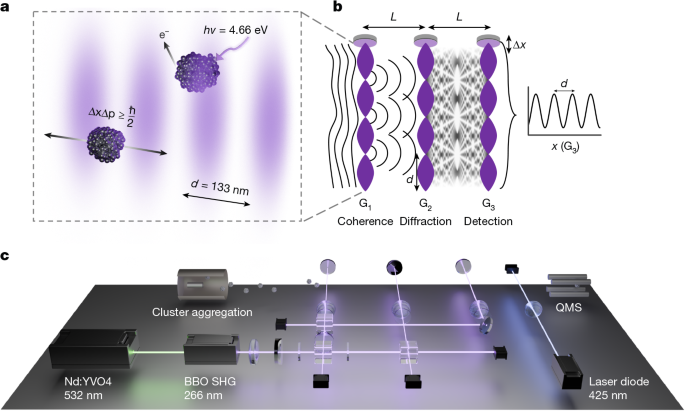
Large sodium clusters are generated in a custom-built aggregation chamber, inspired by earlier work32,59. The sodium is evaporated at 650–700 K into a cold mixture of argon and helium at a liquid nitrogen temperature of 77 K and pressure of less than 1 mbar. The resulting distribution covers masses beyond 1 MDa and velocities between 120 m s−1 and 170 m s−1. The clusters exit through a 5-mm aperture and pass three differential pumping stages before they reach the interferometer (Supplementary Information).
Two horizontal collimation slits dH1,H2 = 0.5 mm spaced by 1.8 m facilitate the alignment of the grating yaw angles perpendicular to the molecular beam with a precision of about 200 μrad. Two vertical collimation slits dV1 = 0.5 mm and dV2 = 1 mm, spaced by 2.2 m, confine the beam height and ensure good overlap with the standing light wave. This also reduces the influence of gravitationally induced phase averaging.
Photophysics
The optical polarizability α266, absorption cross-section σabs,266 and ionization potential Ei depend on the size, mass and purity of the cluster. They determine transmission, the maximal matter-wave phase shift ϕ0 and the mean number of absorbed photons n0 in the antinodes of the grating. Photophysics60 and thermodynamics61 of small sodium clusters have been extensively studied, and the preparation of particles up to 1 MDa has been demonstrated before59. However, the mass-selected UV polarizability has not been known. Here, we use the high-contrast fringe patterns of clusters between 0.4 MDa and 1 MDa to determine it in a mass range for which the classical and quantum models predict the same visibilities. We derive a value of α266/atom = −4πε0 × (4.5 ± 0.5) Å3 (Supplementary Information), which is consistent with the experiments and the quantum model for m = 100–200 kDa.
The photo-ionization cross-section σion,266 is a product of the absorption cross-section σabs,266 and the ionization yield. It determines the total transmission through the interferometer and influences the highest possible interference contrast. By measuring the mass-selected transmission of the interferometer for different grating powers, we determine an effective cross-section of σion,266 = (0.537 × m [kDa] − 1.5) × 10−20 m2 for our clusters.
Mass selection and detection
After passing all gratings, the cluster beam is photo-ionized using 425 nm light and the cations are filtered by their m/z ratio using a quadrupole mass spectrometer. The mass filter includes guiding ion optics (Extrel) and 300 mm long quadrupole rods (Oxford Applied Research) with a diameter of 25.4 mm. The mass filter is operated at a resolution of Δm/m = 0.32. Interference scans centred on mass m, therefore, involve clusters within a mass range of ±Δm/2, where the transmission function is close to rectangular shape and taken into account in our models. The mass filter was centred at 170 kDa. The underlying mass distribution, convoluted with the trapezoidal transmission, shifts the effective mass centre towards 172 kDa.
The selected cluster ions are counted by a channel electron multiplier with a conversion dynode at 10 kV. Electronic dark counts range from 15 to 100 counts s−1.
We must also account for the mixing of multiply charged ions with identical m/z ratios. Based on the measured work function of W = (2.4 ± 0.1) eV (Supplementary Information), neutral clusters with a diameter of dCl ~ 8 nm exhibit an ionization threshold of Ei = 2.53 eV, followed by Ei,+1 = 2.88 eV and Ei,+2 = 3.23 eV for subsequent ionization processes. The detection laser has a photon energy of Eph = 2.92 eV and can generate doubly charged ions, whereas triply charged ions remain energetically out of reach.
We have selected doubly charged clusters in the detector and verified the correct cluster mass by analysing mass spectra at both low and high detection laser powers (Supplementary Information). In the antinodes of the gratings, the 266 nm light can also lead to multiply charged ions. However, this does not affect the interference pattern, because every ion is removed from the cluster beam by electrostatic deflection, independent of its charge state. Only clusters that remain neutral while passing through all gratings contribute to the final interference pattern.
Velocity distribution
The cluster velocity distribution is determined from a time-of-flight measurement, in which we imprint a start time signal onto the cluster beam by UV photodepletion close to G1, and we measure the cluster arrival time behind the ionizing mass spectrometer. The time-of-flight data are corrected for the drift time inside the quadrupole, where it is slightly accelerated by the entrance voltage U to \(v{\prime} =v+\sqrt{2eU\,/\,m}\). A convolution of a Gaussian drift time distribution and a rectangular chopper opening function is then fitted to the corrected unsmoothed data. The results are converted to a velocity distribution. We determine the average velocity and the width of the distribution from the standard deviation of the Gaussian fit.
Small variations of the mean velocity depend on the gas flow and the particle mass, and the 1σ width is Δv/v = 5–7%. Time-of-flight and velocity spectra for m/z = 100 kTh clusters are shown in the Supplementary Information.
Deep ultraviolet gratings
Up to 4 W of 532 nm light (Coherent Verdi V18) is converted to up to 1 W of 266 nm UV light by intracavity second harmonic generation (Sirah Wavetrain 2). The UV output is vertically expanded and split into three grating beams, using polarizing beam splitters and half-wave plates to regulate the power for each grating. Cylindrical lenses (f = 140 mm) focus the laser horizontally onto high-reflectivity (R = 99.5%) mirrors in vacuum to generate the standing light waves. We have observed power losses of up to 60% because of the degradation of optical components. The beam waists before the lenses are W1 × H1 = 1,130 × 620 μm2, W2 × H2 = 1,020 × 575 μm2 and W3 × H3 = 1,020 × 575 μm2, with ΔHi = ΔWi = ±50 μm. Here, Wi represents the 1/e2 waist radii along the molecular beam direction and Hi is the vertical waist. At the focus, the Gaussian beam waist is 20 μm. This small waist alleviates the alignment requirements with regard to the cluster beam tilt angle. The waist is still sufficiently large to ensure that the Rayleigh length, zR = 4.7 mm, is an order of magnitude larger than the cluster beam width of 500 μm.
Interferometer alignment
The surfaces of all three grating mirrors are aligned parallel to the particle beam axis, with the standing light wave along the mirror normal. The gratings exhibit three angular degrees of freedom: pitch, yaw and roll. The yaw angle, between the mirror surface and the particle beam, is adjusted to better than 200 μrad. The relative roll of the three mirrors, that is, their rotation around the axis parallel to the cluster beam is aligned to a difference less than 20 μrad. They are all stabilized with respect to the gravitational field of Earth to better than 50 μrad. The distances between the gratings are equal within 50 μm.
Interference scans
We obtain the interference scans by measuring the number of transmitted clusters as a function of the transverse displacement of the third grating G3, which is moved in steps of Δx = 15 nm. At each position, the mass-filtered ion signal is integrated for a time interval of up to four seconds. A sinusoidal fit to the data then provides the periodicity, phase and amplitude of the fringes. By design of first-order Talbot–Lau interferometry, the periodicity is equal to the grating period. Each visibility \({{\mathcal{V}}}_{i}\) results from a nonlinear least-squares sine fit to the raw counts and is accompanied by 1σ confidence bounds \(({{\mathcal{V}}}_{i,{\rm{lb}}},{{\mathcal{V}}}_{i,{\rm{ub}}})\). We define side-specific absolute uncertainties \({\sigma }_{i,-}={{\mathcal{V}}}_{i}-{{\mathcal{V}}}_{i,{\rm{lb}}}\), \({\sigma }_{i,+}={{\mathcal{V}}}_{i,{\rm{ub}}}-{{\mathcal{V}}}_{i},\) and the effective symmetric uncertainty \({\sigma }_{i}=({\sigma }_{i,-}+{\sigma }_{i,+})/2\). Measurements are grouped by optical power into bins. For each bin \({\mathcal{B}}\), we compute the inverse-variance weighted mean \(\mu ={\sum }_{i\in {\mathcal{B}}}{w}_{i}{{\mathcal{V}}}_{i}/\,{\sum }_{i\in {\mathcal{B}}}{w}_{i}\) with \({w}_{i}={\sigma }_{i}^{-2}\), and to display mild asymmetry, we also report \({\sigma }_{\mu ,-}^{-2}={\sum }_{i\in {\mathcal{B}}}{\sigma }_{i,-}^{-2}\) and \({\sigma }_{\mu ,+}^{-2}={\sum }_{i\in {\mathcal{B}}}{\sigma }_{i,+}^{-2}\). As a consistency check, we compute the reduced chi-square \({\chi }_{{\rm{red}}}^{2}\) using the same per-point uncertainties as the weights. For overdispersed bins (\({\chi }_{{\rm{red}}}^{2} > 1.5\)), we scale the upper and lower error bars of the mean by \(\sqrt{{\chi }_{{\rm{red}}}^{2}}\). For visualization, plotted lower bounds are truncated at 0; all weighting and dispersion checks use the untruncated values.