
The aim of this section is to provide intuition for the main technical contributions of our approach as well as the main difficulties we had to avoid on the way to establishing a generalized quantum Sanov’s theorem, together with its equivalence with the exponent of entanglement distillation under non-entangling operations. Full technical proofs can be found in Supplementary Notes A–E.
Equivalence between entanglement distillation and entanglement testing
Recall that our main object of study is the Sanov exponent \({\rm{S}}{\rm{a}}{\rm{n}}{\rm{o}}{\rm{v}}({\rho }_{AB}\| {{\mathcal{S}}}_{A:B})\). To express this exponent in a convenient way, we will use the hypothesis testing relative entropy53,54
$${D}_{{\rm{H}}}^{\varepsilon }(\sigma \| \rho )\,:=-{\log }_{2}\,\min \{{\rm{T}}{\rm{r}}\,M\rho \,|\,0\le M\le {\mathbb{1}},\,{\rm{T}}{\rm{r}}({\mathbb{1}}-M)\sigma \le \varepsilon \}.$$
(6)
By thinking of M as an arbitrary measurement operator—an element of a POVM—we can understand \((M,{\mathbb{1}}-M)\) as the most general two-outcome measurement that we may use to discriminate between ρ and σ. Assigning the first outcome of this measurement to the state σ and the second to ρ, \({D}_{{\rm{H}}}^{\varepsilon }(\sigma \parallel \rho )\) then precisely quantifies the optimal type I error exponent of hypothesis testing when the type II error probability is constrained to be at most ε. We can then write
$${\rm{S}}{\rm{a}}{\rm{n}}{\rm{o}}{\rm{v}}({\rho }_{AB}\| {{\mathcal{S}}}_{A:B}):=\mathop{\mathrm{lim}}\limits_{\varepsilon \to 0}\mathop{{\rm{l}}{\rm{i}}{\rm{m}}\,{\rm{i}}{\rm{n}}{\rm{f}}}\limits_{n\to \infty }\frac{1}{n}{D}_{{\rm{H}}}^{\varepsilon }\big({{\mathcal{S}}}_{{A}^{n}:{B}^{n}}\|\,{\rho }_{AB}^{\otimes n}\big),$$
(7)
where we note that the optimized hypothesis testing relative entropy can be written as
$$\begin{array}{rcl}{D}_{{\rm{H}}}^{\varepsilon }({{\mathcal{S}}}_{A:B}\| {\rho }_{AB}) & = & \mathop{\min }\limits_{\sigma \in {{\mathcal{S}}}_{A:B}}{D}_{{\rm{H}}}^{\varepsilon }({\sigma }_{AB}\| {\rho }_{AB})\\ & = & -{\log }_{2}\,\min \{{\rm{T}}{\rm{r}}M{\rho }_{AB}\,|\,0\!\le\! M\!\le\! {\mathbb{1}},\,{\rm{T}}{\rm{r}}\,M\sigma \!\ge\! 1\!-\!\varepsilon\ {\rm{\forall }}\,\sigma \in {{\mathcal{S}}}_{A:B}\},\end{array}$$
(8)
with the equality on the second line following from von Neumann’s minimax theorem55.
We remark here that the name ‘Sanov’s theorem’ is typically used in the classical information theory literature to refer to a slightly different result on the probability of observing samples whose empirical distribution (type) lies in a given set of distributions (Section 11.4 of ref. 56). We follow other works in quantum information theory, starting with ref. 33, which used the name ‘quantum Sanov’s theorem’ to refer to a hypothesis testing problem with a composite null hypothesis, like (but not directly comparable with) the setting we study here. We specifically use the name ‘generalized quantum Sanov’s theorem’ because our composite hypothesis testing problem involves a general set of non-i.i.d. states \({{\mathcal{S}}}_{{A}^{n}:{B}^{n}}\), in the same way that the ‘generalized quantum Stein’s lemma’ is now commonly used to refer to the closely related composite setting introduced in ref. 7. The same generalized variant of quantum Sanov’s theorem was previously studied in ref. 9, where only bounds on the optimal asymptotic exponent were obtained (see also section ‘On entropies and their (non-)additivity’). Yet another quantum variant of Sanov’s theorem, more closely related to the original formulation of classical Sanov’s theorem based on empirical distributions, was recently proposed by Hayashi57; this, however, is not directly related to the setting studied here.
The claim of our Lemma 1 is the asymptotic equivalence between this quantity and the error exponent of entanglement distillation, which we recall to be
$${E}_{{\rm{d}},{\rm{e}}{\rm{r}}{\rm{r}}}({\rho }_{AB})=\mathop{\mathrm{lim}}\limits_{m\to \infty }{E}_{{\rm{d}},{\rm{e}}{\rm{r}}{\rm{r}}}^{(m)}({\rho }_{AB}),$$
(9)
where \({E}_{{\rm{d}},{\rm{e}}{\rm{r}}{\rm{r}}}^{(m)}\) denotes the exponent of distillation under non-entangling operations for a fixed number of m output copies:
$${E}_{{\rm{d}},{\rm{e}}{\rm{r}}{\rm{r}}}^{(m)}({\rho }_{AB}):=\sup \Big\{\mathop{{\rm{l}}{\rm{i}}{\rm{m}}\,{\rm{i}}{\rm{n}}{\rm{f}}}\limits_{n\to \infty }-\frac{1}{n}{\log }_{2}\,{\varepsilon }_{n}\,\Big|\, {{{\Lambda }}}_{n}(\rho^{\otimes n}_{AB}){\approx }_{{\varepsilon }_{n}}| {\varPhi }_{+}\rangle {\langle {\varPhi }_{+}| }^{\otimes m},\,{\varLambda }_{n}\in {\rm{N}}{\rm{E}}\Big\},$$
(10)
where the supremum is understood to be over all sequences \({({\varLambda }_{n})}_{n\in {{{\mathbb{N}}}}}\) of operations satisfying the specified constraints and, in particular, belonging to the class of non-entangling maps.
We now outline the main part of our argument, the details of which can be found in Supplementary Note A. The approach bears some technical similarity with a construction used in ref. 36, but a crucial difference is that we employ the connection in a rather different way. Instead of the type II hypothesis-testing error, which was the object of study in ref. 36, we are interested in the type I error, and suitable modifications of the proof have to be made to account for this. This shift is what distinguishes our approach and ultimately leads to quantitatively different results.
On the one hand, any distillation protocol \({({\varLambda }_{n})}_{n}\) can be turned into a suitable sequence of tests \(({M}_{n},{\mathbb{1}}-{M}_{n})\) that perform entanglement testing with a small type I error probability. Because \({\varLambda }_{n}({\rho }_{AB}^{\otimes n})\)\({\approx }_{{\varepsilon }_{n}} |{\varPhi }_{+}\rangle {\langle {\varPhi }_{+}| }^{\otimes m}\), we can construct a measurement by defining \({M}_{n}\,:={\mathbb{1}}-{\varLambda }_{n}^{\dagger }(| {\varPhi }_{+}\rangle {\langle {\varPhi }_{+}| }^{\otimes m})\), where \({\varLambda }_{n}^{\dagger }\) denotes the adjoint map of Λn. This represents the action of the channel in the Heisenberg picture. We can then show that the type II error probability of this test is at most 2−m, whereas the type I error is at most εn; this gives a feasible protocol for entanglement testing, leading to the bound
$$\mathop{\min }\limits_{{\sigma }_{n}\in {{\mathcal{S}}}_{{A}^{n}:{B}^{n}}}{D}_{{\rm{H}}}^{{2}^{-m}}\big({\sigma }_{n}\, \|\, {\rho }_{AB}^{\otimes n}\big)\ge {\log }_{2}\frac{1}{{\rm{T}}{\rm{r}}\,{M}_{n}{\rho }_{AB}^{\otimes n}}\ge -{\log }_{2}{\varepsilon }_{n},$$
(11)
which is one direction of the claimed relation.
For the other direction, we take any sequence of feasible measurement operators Mn for entanglement testing of \({\rho }_{AB}^{\otimes n}\) and use them to construct a distillation protocol. This is done through a simple measure-and-prepare procedure: we first perform the measurement \(({M}_{n},{\mathbb{1}}-{M}_{n})\), and if we obtain the first outcome (we think that the input state is separable), then we simply prepare a suitable separable state; if, however, we obtain the second outcome (we think that the state is \({\rho }_{AB}^{\otimes n}\)), then we prepare our desired target state \({| {\varPhi }_{+}\rangle }^{\otimes m}\). In Supplementary Note A we show that this constitutes a feasible distillation protocol with error \({\varepsilon }_{n}=\mathrm{Tr}\,{M}_{n}{\rho }_{AB}^{\otimes n}\), giving
$${E}_{{\rm{d}},{\rm{e}}{\rm{r}}{\rm{r}}}^{(m)}({\rho }_{AB})\ge \mathop{{\rm{l}}{\rm{i}}{\rm{m}}\,{\rm{i}}{\rm{n}}{\rm{f}}}\limits_{n\to \infty }\frac{1}{n}\mathop{\min }\limits_{{\sigma }_{n}\in {{\mathcal{S}}}_{{A}^{n}:{B}^{n}}}{D}_{{\rm{H}}}^{{2}^{-m}}\big({\sigma }_{n}\,\|\, {\rho }_{AB}^{\otimes n}\big).$$
(12)
Altogether the above arguments show that
$$\begin{array}{cl}{E}_{{\rm{d}},\mathrm{err}}({\rho }_{AB}) & =\mathop{\mathrm{lim}}\limits_{m\to \infty }{E}_{{\rm{d}},\mathrm{err}}^{(m)}(\rho )=\mathop{\mathrm{lim}}\limits_{m\to \infty }\mathop{\mathrm{lim}\,\inf }\limits_{n\to \infty }\displaystyle\frac{1}{n}\mathop{\min }\limits_{{\sigma }_{n}\in {{\mathcal{S}}}_{{A}^{n}:{B}^{n}}}{D}_{{\rm{H}}}^{{2}^{-m}}\big({\sigma }_{n}\,\|\, {\rho }_{AB}^{\otimes n}\big)\\ & =\mathrm{Sanov}({\rho }_{AB}\| {{\mathcal{S}}}_{A:B}),\end{array}$$
(13)
which establishes an equivalence between the error exponent of entanglement distillation and the Sanov exponent of entanglement testing.
On entropies and their (non-)additivity
Let us now consider the claim of our main result, namely, that \({\rm{S}}{\rm{a}}{\rm{n}}{\rm{o}}{\rm{v}}({\rho }_{AB}\| {{\mathcal{S}}}_{A:B})=D({{\mathcal{S}}}_{A:B}\| {\rho }_{AB})\).
A simple but key observation that helps motivate this claim is that the reverse relative entropy of entanglement is, in fact, additive on tensor product states35. That is, we have
$$D({{\mathcal{S}}}_{A{A}^{{\prime} }:B{B}^{{\prime} }}\| {\rho }_{AB}\otimes {\omega }_{{A}^{{\prime} }{B}^{{\prime} }})=D({{\mathcal{S}}}_{A:B}\| {\rho }_{AB})+D({{\mathcal{S}}}_{{A}^{{\prime} }:{B}^{{\prime} }}\| {\rho }_{{A}^{{\prime} }{B}^{{\prime} }})$$
(14)
for all states ρAB and \({\omega }_{{A}^{{\prime} }{B}^{{\prime} }}\). To see this, let \({\sigma }_{A{A}^{{\prime} }B{B}^{{\prime} }}\in {{\mathcal{S}}}_{A{A}^{{\prime} }:B{B}^{{\prime} }}\) be a minimizer of \(D({{\mathcal{S}}}_{A{A}^{{\prime} }:B{B}^{{\prime} }}\| {\rho }_{AB}\otimes {\omega }_{{A}^{{\prime} }{B}^{{\prime} }})\), and use that \({\log }_{2}({\rho }_{AB}\otimes {\omega }_{{A}^{{\prime} }{B}^{{\prime} }})\)\(={\log }_{2}\,{\rho }_{AB}\otimes {{\mathbb{1}}}_{A’B’}\)\(+{{\mathbb{1}}}_{AB}\otimes {\log }_{2}\,{\omega }_{A’B’}\) to get
$$\begin{array}{cl}D({\sigma }_{A{A}^{{\prime} }B{B}^{{\prime} }}\| {\rho }_{AB}\otimes {\omega }_{{A}^{{\prime} }{B}^{{\prime} }}) & =-S({\sigma }_{A{A}^{{\prime} }B{B}^{{\prime} }})+D({\sigma }_{AB}\| {\rho }_{AB})\\ & \quad\; +D({\sigma }_{{A}^{{\prime} }{B}^{{\prime} }}\| {\omega }_{AB})+S({\sigma }_{AB})+S({\sigma }_{{A}^{{\prime} }{B}^{{\prime} }})\\ & =I{(A{A}^{{\prime} }:B{B}^{{\prime} })}_{\sigma }+D({\sigma }_{AB}\| {\rho }_{AB})+D({\sigma }_{{A}^{{\prime} }{B}^{{\prime} }}\| {\omega }_{AB})\\ & \ge D({{\mathcal{S}}}_{A:B}\| {\rho }_{AB})+D({{\mathcal{S}}}_{{A}^{{\prime} }:{B}^{{\prime} }}\| {\omega }_{{A}^{{\prime} }{B}^{{\prime} }}),\end{array}$$
(15)
where the last line follows from the non-negativity of the quantum mutual information \(I{(A{A}^{{\prime} }:B{B}^{{\prime} })}_{\sigma }=S({\sigma }_{AB})+S({\sigma }_{{A}^{{\prime} }{B}^{{\prime} }})-S({\sigma }_{A{A}^{{\prime} }B{B}^{{\prime} }})\) (Theorem 11.6.1 in ref. 58) and the fact that the reduced systems σAB and \({\sigma }_{{A}^{{\prime} }{B}^{{\prime} }}\) are always separable for \({\sigma }_{A{A}^{{\prime} }B{B}^{{\prime} }}\) separable between \(A{A}^{{\prime} }\) versus \(B{B}^{{\prime} }\). This already tells us that this quantity can help us avoid issues with many-copy formulas, as regularization is simply not needed for this formula.
Although the converse direction \({\rm{S}}{\rm{a}}{\rm{n}}{\rm{o}}{\rm{v}}({\rho }_{AB}\| {{\mathcal{S}}}_{A:B})\le D({{\mathcal{S}}}_{A:B}\| {\rho }_{AB})\) can straightforwardly be concluded from the converse of the standard i.i.d. setting, for the other direction, we need to construct a composite hypothesis test that works well enough to distinguish any separable state from \({\rho }_{AB}^{\otimes n}\). Now, consider first a simpler case: if we were to test against a fixed tensor product state \({\sigma }_{AB}^{\otimes n}\) instead of the whole set of separable states, the quantum Stein’s lemma27 would immediately tell us that D(σAB∥ρAB) is an achievable error exponent. In more detail, the modern and arguably simplest approach for proving the achievability part of i.i.d. quantum hypothesis testing goes through the family of Petz–Rényi divergences\({D}_{\alpha }(\sigma \| \rho )=\frac{1}{\alpha -1}{\log }_{2}\,{\rm{T}}{\rm{r}}\,{\sigma }^{\alpha }{\rho }^{1-\alpha }\) (ref. 59), which leads via Audenaert et al.’s inequality60 to
$${\rm{S}}{\rm{a}}{\rm{n}}{\rm{o}}{\rm{v}}({\rho }_{AB}\| {\sigma }_{AB})\ge \displaystyle \mathop{\mathrm{lim}}\limits_{\alpha \to {1}^{-}}\mathop{\mathrm{lim}}\limits_{n\to \infty }\frac{1}{n}{D}_{\alpha }\big({\sigma }_{AB}^{\otimes n}\,\|\, {\rho }_{AB}^{\otimes n}\big)=D({\sigma }_{AB}\| {\rho }_{AB}).$$
(16)
Here the crucial point in the derivation is that \({D}_{\alpha }\big({\sigma }_{AB}^{\otimes n}\,\big\| \,{\rho }_{AB}^{\otimes n}\big)\)\(=n{D}_{\alpha }({\sigma }_{AB}\|\, {\rho }_{AB})\) is an additive bound on the error probability that becomes asymptotically tight with \({\mathrm{lim}}_{\alpha \to {1}^{-}}{D}_{\alpha }({\sigma }_{AB}\|\, {\rho }_{AB})\)\(=D({\sigma }_{AB}\| \,{\rho }_{AB})\) (ref. 59). One might then wonder whether these state-of-the-art quantum hypothesis-testing methods could also be used for the generalized Sanov’s theorem, where the fixed state \({\sigma }_{AB}^{\otimes n}\) is replaced with the set of states \({{\mathcal{S}}}_{A{:}B}\).
Indeed, this approach was recently initiated in ref. 9, and consequently, the question was raised whether the corresponding Petz–Rényi divergences of entanglement \({D}_{\alpha }({{\mathcal{S}}}_{A:B}\|\, {\rho }_{AB})\) become additive. Perhaps surprisingly, however, we can show that, in contrast to the aforementioned special case α = 1, the divergences are not additive for α ∈ (0, 1). Namely, by taking the antisymmetric Werner state ρa as an example, it can be shown that61 (Supplementary Note E)
$${D}_{\alpha }({{\mathcal{S}}}_{A{A}^{{\prime} }:B{B}^{{\prime} }}\| {\rho }_{{\rm{a}}}\otimes {\rho }_{{\rm{a}}}) < 2{D}_{\alpha }({{\mathcal{S}}}_{A:B}\| {\rho }_{{\rm{a}}}).$$
(17)
This non-additivity means that, to characterize the generalized Sanov exponent, we would really need to work with the regularized quantities \({\mathrm{lim}}_{n\to \infty }\frac{1}{n}{D}_{\alpha }\big({{\mathcal{S}}}_{{A}^{n}:{B}^{n}}\,\|\, {\rho }_{AB}^{\otimes n}\big)\). Unfortunately, this prevents us from being able to use the known continuity results for the Petz–Rényi divergences (cf. refs. 8,9) and makes it difficult to follow the approach of ref. 9 to establish a connection with the reverse relative entropy \(D({{\mathcal{S}}}_{A:B}\| {\rho }_{AB})\), which is our goal. As such, we need to overcome this technical bottleneck in known proof techniques and develop an approach that will allow us to resolve the generalized Sanov’s theorem.
Axiomatic approach
Recall that our main goal is to characterize the asymptotic error exponent in entanglement testing, that is, distinguishing a sequence of states \({\rho }_{AB}^{\otimes n}\) from the set of separable states \({{\mathcal{S}}}_{A:B}\). However, it will be useful to forget about separable states for now and try to understand the set in an axiomatic manner, using only some of its basic properties. Such an axiomatic approach is due to the influential works of Brandão and Plenio7 in connection with the generalized quantum Stein’s lemma (cf. the recent works in refs. 8,10,11).
This has a dual purpose: on the one hand, it will immediately allow us to apply many of our results to quantum resource theories beyond entanglement32,62; more importantly, however, it will actually also be a crucial ingredient in our proof of the generalized quantum Sanov’s theorem for entanglement theory itself.
To do this, let us work out a list of abstract mathematical properties obeyed by the set of separable states as well as by other relevant sets of free states. The first five of these properties were proposed by Brandão and Plenio7 and are sometimes known as the Brandão–Plenio axioms. To state them, we consider some quantum system with Hilbert space \({\mathcal{H}}\) and a sequence \({({{\mathcal{F}}}_{n})}_{n}\) of sets \({{\mathcal{F}}}_{n}\subseteq {\mathcal{D}}({{\mathcal{H}}}^{\otimes n})\) of density operators on n copies of \({\mathcal{H}}\). States in \({{\mathcal{F}}}_{n}\) are conventionally referred to as free states, and a state that is not free is called resourceful. We posit the following axioms:
1.
For each n, \({{\mathcal{F}}}_{n}\) is a convex and closed subset of states.
2.
\({{\mathcal{F}}}_{1}\) contains some full-rank state σ0 > 0, for example, the maximally mixed state.
3.
The family \({({{\mathcal{F}}}_{n})}_{n}\) is closed under partial traces: tracing out any number of the n subsystems cannot make a free state resourceful.
4.
The family \({({{\mathcal{F}}}_{n})}_{n}\) is closed under tensor products: the tensor product of any two free states is also free.
5.
Each \({{\mathcal{F}}}_{n}\) is closed under permutations: permuting any of the n subsystems cannot create a resource from a free state.
Picking \({\mathcal{H}}={{\mathcal{H}}}_{AB}={{\mathcal{H}}}_{A}\otimes {{\mathcal{H}}}_{B}\) as a bipartite Hilbert space and taking \({{\mathcal{F}}}_{n}={{\mathcal{S}}}_{{A}^{n}:{B}^{n}}\) as the set of separable states on \({{\mathcal{H}}}_{A}^{\otimes n}\otimes {{\mathcal{H}}}_{B}^{\otimes n}\) (with all A systems on one side and all B systems on the other) clearly satisfies all of the above Axioms 1–5. However, these axioms are also obeyed by many other sets of free states, corresponding to different quantum resource theories62. All of our definitions can be immediately extended to such sets, with the conjectured generalized Sanov’s theorem now asking whether
$${\rm{S}}{\rm{a}}{\rm{n}}{\rm{o}}{\rm{v}}(\rho \| {\mathcal{F}})\mathop{=}\limits^{?}D({\mathcal{F}}\| \rho )=\mathop{\min }\limits_{\sigma \in {{\mathcal{F}}}_{1}}D(\sigma \| \rho )\,.$$
(18)
Although the above natural set of axioms, indeed, turns out to be sufficient to prove the generalized quantum Stein’s lemma10,11, note that the axioms are not sufficient for the generalized Sanov’s theorem. In Supplementary Note E we give a classical example that fulfils Axioms 1–5, while anyway having
$${\rm{S}}{\rm{a}}{\rm{n}}{\rm{o}}{\rm{v}}(\rho \| {\mathcal{F}})=0 < \infty =D({\mathcal{F}}\| \rho )$$
(19)
for some (classical) state ρ. To remedy this problem, we need to introduce a further assumption about the sets \({{\mathcal{F}}}_{n}\). We first consider the following extra axiom:
6.
The regularized relative entropy of resource is faithful. That is, for all resourceful \(\rho \in {\mathcal{D}}({\mathcal{H}})\) with \(\rho \notin {{\mathcal{F}}}_{1}\), we have that \({D}^{\infty }(\rho \,\| \,{\mathcal{F}})\)\(:\!={\mathrm{lim}}_{n\to \infty }\frac{1}{n}\,D({\rho }^{\otimes n}\,\| \,{{\mathcal{F}}}_{n}) > 0\).
We note here that this concerns the conventional definition of the relative entropy \({D}^{\infty }(\rho \| {\mathcal{F}})\) rather than the ‘reverse’ variant \(D({\mathcal{F}}\| \rho )\). This rather non-trivial property is obeyed by many quantum resources encountered in practice. For instance, for separable states, it has been proved to hold independently by Brandão and Plenio (Corollary II.2 in ref. 7) and by Piani63. It is, however, not universal, and the counterexample in equation (19) violates this axiom. Indeed, Axiom 6 turns out to be sufficient, together with Axioms 1–5, to imply the generalized Sanov theorem in the fully classical case. That is, instead of general quantum states, we restrict ourselves to classical probability distributions (commuting states). However, the axiom does not seem to suffice to establish the quantum extension of this finding. To derive the quantum result, we will, instead, need an axiom that is seemingly rather different from Axiom 6 but actually closely related to it. This new Axiom 6’ is concerned with how measurements close to the identity act on the set of free states:
6′. For some choice of numbers \({r}_{n}\in (0,1]\), the sequence \({({{\mathbb{M}}}_{n})}_{n}\) of sets of measurements
$${{\mathbb{M}}}_{n\,}:=\left\{\left(\frac{{{\mathbb{1}}}^{\otimes n}+{X}_{n}}{2},\,\frac{{{\mathbb{1}}}^{\otimes n}-{X}_{n}}{2}\right):\,{X}_{n}={X}_{n}^{\dagger }\in {\mathcal{L}}({{\mathcal{H}}}^{\otimes n}),\,\parallel \!{X}_{n}{\parallel }_{\infty }\le {r}_{n}\right\},$$
(20)
where ∥ ⋅ ∥∞ denotes the operator norm, is compatible with \({({{\mathcal{F}}}_{n})}_{n}\) (refs. 42,63). This means that whenever a measurement \({\mathcal{M}}\in {{\mathbb{M}}}_{n}\) is performed on the first n subsystems of a free state \(\sigma \in {{\mathcal{F}}}_{n+m}\), the resulting post-measurement state on the last m subsystems is also a free state in \({{\mathcal{F}}}_{m}\) for each one of the two possible outcomes of \({\mathcal{M}}\). Here, \(\mathcal{L}({\mathcal{H}}^{\otimes n})\) denotes the space of linear operators acting on the Hilbert space \({\mathcal{H}}^{\otimes n}\).
Aside from the fact that both are obeyed by the set of separable states, as we show in Supplementary Note D, it is a priori unclear why Axiom 6’ is in any way related to Axiom 6. The connection between the two follows from the work of Piani63, who proved that Axiom 6 is satisfied whenever one can find a tomographically complete set of measurements that is compatible with the free states; the sets \({{\mathbb{M}}}_{n}\) in equation (20) are, in fact, tomographically complete because the POVM operators \(({{\mathbb{1}}}^{\otimes n}+{X}_{n})/2\) span the space of Hermitian operators on \({{\mathcal{H}}}^{\otimes n}\). It turns out that Axiom 6’ is what we need to prove the generalized quantum Sanov’s theorem.
In the following, our proof strategy will be to:
(1)
Derive the generalized Sanov’s theorem for the commutative case of sets of classical states \({{\mathcal{F}}}_{n}\) that respect Axioms 1–6 (sections ‘Max-relative entropy and the blurring lemma’ and ‘Classical generalized Sanov’s theorem’).
(2)
Choose suitable measurement operations for lifting the result to the non-commutative (quantum) setting, assuming Axioms 1–5 as well as Axiom 6’ (section ‘Lifting from classical to quantum’).
Max-relative entropy and the blurring lemma
Instead of directly working with the hypothesis-testing relative entropy \({D}_{{\rm{H}}}^{\varepsilon }(\sigma \| \rho )\), our proofs start with a dual formulation in terms of the smooth max-relative entropy, which is defined as
$${D}_{\max }^{\varepsilon }(\sigma \| \rho ):={\log }_{2}\,\inf \Big\{\mu \in {\mathbb{R}}\,\Big| \,\widetilde{\sigma }\le \mu \rho ,\,\frac{1}{2}\| \widetilde{\sigma }-\sigma {\| }_{1}\le \varepsilon \Big\},$$
(21)
where we choose to measure the ε-closeness of states in terms of the trace distance. The smooth max-relative entropy enjoys, for any δ > 0 small enough, the duality relation64,65,66
$${D}_{\max }^{\sqrt{1-\varepsilon }}(\sigma \| \rho )\le {D}_{{\rm{H}}}^{\varepsilon }(\sigma \| \rho )\le {D}_{\max }^{1-\varepsilon -\delta }(\sigma \| \rho )+{\log }_{2}\frac{1}{\delta },$$
(22)
which implies that we can essentially replace the hypothesis-testing relative entropy with the smooth max-relative entropy, up to suitably modifying the smoothing parameter.
The generalized Sanov’s theorem for general sets of states \({\mathcal{F}}\) then becomes equivalent to
$$\displaystyle \mathop{\mathrm{lim}}\limits_{n\to \infty }\frac{1}{n}\,{D}_{\max }^{\varepsilon }({{\mathcal{F}}}_{n}\,\| \,{\rho }^{\otimes n})\mathop{=}\limits^{?}D({\mathcal{F}}\| \rho )\quad\forall \,\varepsilon \in (0,1),$$
(23)
and, using standard entropic arguments, it is not too difficult to show the special case ε → 0. Further, because the function on the left-hand side of equation (23) is monotonically non-increasing in ε, we immediately have that \({\mathrm{lim}}_{n\to \infty }\frac{1}{n}\,{D}_{\max }^{\varepsilon }({{\mathcal{F}}}_{n}\,\| \,{\rho }^{\otimes n})\le D({\mathcal{F}}\| \rho )\); consequently, it remains to prove the opposite direction. By contradiction, our goal will be to show for the classical case that
$$\frac{1}{n}\,{D}_{\max }^{\varepsilon }({{\mathcal{F}}}_{n}\,\| \,{p}^{\otimes n})\mathop{\longrightarrow }\limits_{n\to \infty }\lambda < D({\mathcal{F}}\| p),$$
(24)
under the assumption of Axioms 1–6.
The crucial tool for working with classical non-i.i.d. distributions in \({{\mathcal{F}}}_{n}\) is the blurring lemma recently established by one of us11. Namely, for any pair of positive integers \(n,m\in {{\mathbb{N}}}_{+}\), one defines the blurring map \({B}_{n,m}:{{\mathbb{R}}}^{{{\mathcal{X}}}^{n}}\to {{\mathbb{R}}}^{{{\mathcal{X}}}^{n}}\), which transforms any input probability distribution by adding m symbols of each kind \(x\in {\mathcal{X}}\), where \(X\) is a a finite alphabet, shuffling the resulting sequence and discarding m symbols.
To better understand the action of this map, it is useful to recall some concepts from the theory of types67. The type of a sequence xn of n symbols from a finite alphabet \({\mathcal{X}}\), denoted \({t}_{{x}^{n}}\), is simply the empirical probability distribution of the symbols of \({\mathcal{X}}\) found in xn: in other words, \({t}_{{x}^{n}}(x)=\frac{1}{n}\,N(x| {x}^{n})\), where N(x∣xn) denotes the number of times x appears in the sequence xn. The set of n-types is denoted as \({{\mathcal{T}}}_{n}\) (we regard the alphabet as fixed). A standard counting argument reveals that the number of types is only polynomial in n, unlike the number of possible sequences xn, which is exponential. More precisely, we have the estimate \(| {{\mathcal{T}}}_{n}| \le {(n+1)}^{| {\mathcal{X}}| -1}\). This means that the size of the type classes, which comprise the set of sequences of a given type, is generically exponential. In what follows, we will indicate with Tn,t the type class associated with a given n-type \(t\in {{\mathcal{T}}}_{n}\). Clearly, the union of all the type classes reproduces the set of all sequences.
An important observation for us is that any probability distribution pn on \({{\mathcal{X}}}^{n}\) that is invariant under permutations, which means that the probability of two sequences that differ only by the order of the symbols is the same, can be understood in the space of types rather than in the space of sequences. In other words, such a probability distribution is uniquely specified by the values pn(Tn,t) that it assigns to each type class. The essence of the blurring lemma, as stated below in equation (25), is the analysis of the effect that the above blurring map has in type space. As blurring perturbs the type of the input sequence a little in a random way, this action amounts to an effective ‘smearing’ of the input probability distribution in type space: a little of the probability weight that every type class carries ‘spills over’ to neighbouring type classes.
More quantitatively, the classical one-shot blurring lemma from ref. 11 (Lemma 9) then tells us that for δ, η > 0 and \({p}_{n},{q}_{n}\in {\mathcal{P}}({{\mathcal{X}}}^{n})\) permutationally symmetric with \({p}_{n}\big({\bigcup }_{t\in {{\mathcal{T}}}_{n}:\parallel s-t{\parallel }_{\infty }\le \delta }{T}_{n,t}\big)\ge 1-\eta\), we have
$${D}_{\max}^{\eta }({p}_{n}\,\| \,{B}_{n,m}({q}_{n}))\le {\log }_{2}\frac{1}{{q}_{n}({\cup }_{t\in {T}_{n}:\parallel s-t{\parallel }_{\infty }\le \delta }{T}_{n,t})}+ng\left(\left(2\delta +\frac{1}{n}\right)|X|\right),$$
(25)
for m = ⌈2δn⌉ and with the fudge function \(g(x)\,:=(x+1)\,{\log }_{2}(x+1)\)\(-x\,{\log }_{2}x\). Refer to Supplementary Note C for more details and to Lemma 9 in ref. 11 for a detailed technical derivation.
Classical generalized Sanov’s theorem
We will now attempt to give an intuitive but mathematically non-rigorous description of the proof of the classical version of Sanov’s theorem, which states that \({\rm{S}}{\rm{a}}{\rm{n}}{\rm{o}}{\rm{v}}(p\|{\mathcal{F}})=D({\mathcal{F}}\| p)\) under Axioms 1–6 in section ‘Axiomatic approach’. Following section ‘Max-relative entropy and the blurring lemma’ and, in particular, equation (24), by contradiction we can then construct two sequences of ε-close probability distributions \({q}_{n}^{{\prime} },{q}_{n}\), with \({q}_{n}\in {{\mathcal{F}}}_{n}\), such that \({q}_{n}^{{\prime} }\le {2}^{n\lambda }{p}^{\otimes n}\).
To make sense of this inequality, we have to evaluate it on a cleverly chosen set. The key tool for doing that is a simple lemma by Sanov, sometimes also known, alas, as Sanov’s theorem. This tells us that68
$${p}^{\otimes n}(\{{x}^{n}:\,{t}_{{x}^{n}}\in {\mathcal{A}}\})\le {\rm{p}}{\rm{o}}{\rm{l}}{\rm{y}}(n)\,{2}^{-nD({\mathcal{A}}\parallel p)}$$
(26)
for any set of probability distributions \({\mathcal{A}}\). It is clear what to do now: by choosing \({\mathcal{A}}={{\mathcal{F}}}_{1}\), we get on the right-hand side the exponential factor \({2}^{n(\lambda -D({\mathcal{F}}\| p))}\), which goes to zero sufficiently fast to overcome the polynomial. Thus, we have that \({q}_{n}^{{\prime} }(\{{x}^{n}:\,{t}_{{x}^{n}}\in {{\mathcal{F}}}_{1}\})\mathop{\to }\limits_{n\to \infty }0\); in other words, a sequence drawn according to \({q}_{n}^{{\prime} }\) has asymptotically vanishing probability of having a free type, that is, a type in \({{\mathcal{F}}}_{1}\).
This, at first sight, may seem good, but it should make us immediately suspicious, because \({q}_{n}^{{\prime} }\) is supposed to be ε-close to a free probability distribution \({q}_{n}\in {{\mathcal{F}}}_{n}\). It thus holds that \({q}_{n}\big(\{{x}^{n}:\,{t}_{{x}^{n}}\notin {{\mathcal{F}}}_{1}\}\big)\gtrsim 1-\varepsilon\) asymptotically. That is, sequences drawn with respect to the free probability distribution qn have a non-free type with an asymptotically non-vanishing probability.
Let us elaborate on this intuition. As there are only a polynomial number of types, the above reasoning shows that there exists a non-free type \(s\notin {{\mathcal{F}}}_{1}\) such that \({q}_{n}({T}_{n,s})\gtrsim \frac{1-\varepsilon }{\mathrm{poly}(n)} \vphantom{\Big|}\). Of course, s might depend on n, but for now the reader will have to trust us that up to extracting converging subsequences, we can circumvent this obstacle (Supplementary Note C). So, now we have a free probability distribution qn that has a substantial weight (only polynomially vanishing) on a certain type class Tn,s corresponding to a non-free type \(s\notin {{\mathcal{F}}}_{1}\).
Enter blurring. By blurring qn, we can make it have substantial weight not only on Tn,s but on all type classes Tn,t with t ≈ s. This is what blurring does: it spreads weight around among close type classes. Hence, we will have that \({\widetilde{q}}_{n}({T}_{n,t})\gtrsim \frac{1-\varepsilon }{{\rm{p}}{\rm{o}}{\rm{l}}{\rm{y}}(n)\,{2}^{\alpha n}}\) for all t ≈ s, where α > 0 is a very small exponential price we have to pay to blur qn into \({\widetilde{q}}_{n}\). For a more quantitative understanding of this phenomenon, we refer the reader to equation (25) and to the full technical proof in Supplementary Note C.
Now, because \({\widetilde{q}}_{n}\) has substantial weight in a whole neighbourhood of types around s, it becomes ideally suited to dominate probability distributions that are very concentrated there. There is an obvious candidate for one such distribution, and it is s⊗n itself! What this reasoning will eventually show is that
$${s}^{\otimes n}\lesssim \frac{{\rm{p}}{\rm{o}}{\rm{l}}{\rm{y}}(n)\,{2}^{\alpha n}}{1-\varepsilon }\,{\widetilde{q}}_{n},$$
(27)
where in ≲ we have swept under the carpet the fact that s⊗n needs to be deprived of its exponentially vanishing non-typical tails for this entry-wise inequality to work.
Now we are basically done. Because blurring does not increase the max-relative entropy of a resource significantly, it is possible to find a free probability distribution \({r}_{n}\in {{\mathcal{F}}}_{n}\) such that \({\widetilde{q}}_{n}\le {2}^{\beta n}{r}_{n}\) for some small β > 0. Chaining the inequalities will give us
$${s}^{\otimes n}\lesssim \frac{\mathrm{poly}(n)\,{2}^{(\alpha +\beta )n}}{1-\varepsilon }\,{r}_{n}\,,$$
(28)
which, by the asymptotic equipartition property expressed as7,69
$$\mathop{\mathrm{lim}}\limits_{\varepsilon \to 0}\,\mathop{{\mathrm{lim}}\,{\mathrm{inf}}}\limits_{n\to \infty }\frac{1}{n}\,{D}_{\max }^{\varepsilon }({s}^{\otimes n}\|{\mathcal{F}}_{n})=D^{\infty }(s\| {\mathcal{F}}),$$
(29)
eventually implies that \({D}^{\infty }(s\| {\mathcal{F}})=0\). This is in direct contradiction with Axiom 6, and this contradiction will complete the proof.
A full technical proof following the argument sketched above is given in Supplementary Note C.
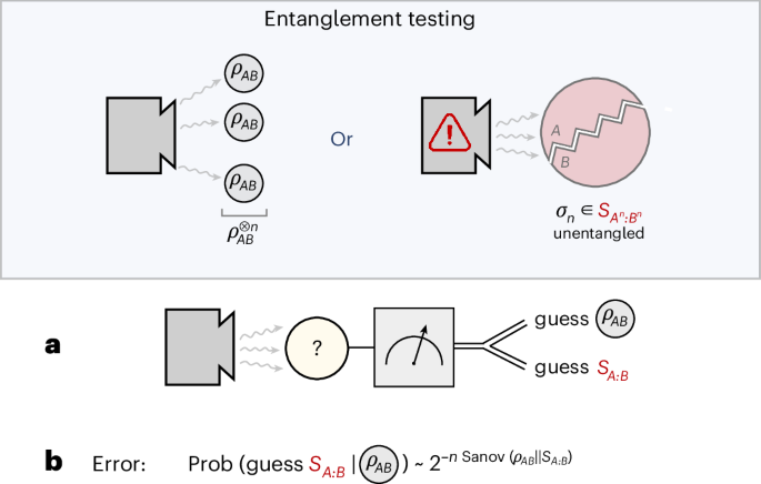
As a by-product of our argument, it is actually possible to design a simple explicit test that is asymptotically nearly optimal for the hypothesis task at hand. Namely, given a string of symbols \({x}^{n}\in {{\mathcal{X}}}^{n}\) and some small tolerance ζ > 0:
If \(\frac{1}{2}{\parallel {t}_{{x}^{n}}-{{\mathcal{F}}}_{1}\parallel }_{1}\le \zeta\), where \({t}_{{x}^{n}}\) is the type of xn, then we guess that the underlying probability distribution is free.
Otherwise, we guess that it is p.
This test can be shown to achieve an asymptotically vanishing type II error probability in the limit when n → ∞ and a type I error exponent that is approximately equal to the reverse relative entropy \(D({\mathcal{F}}\| p)\), if ζ > 0 is sufficiently small.
Lifting from classical to quantum
Once a solution of the classical problem has been established, we need to extend it to quantum systems. To do this, a standard strategy is to measure: indeed, quantum measurements map quantum states to classical probability distributions, so we can use them to bring the problem to a form that we can tackle with our classical result.
In the context of hypothesis testing, and, more specifically, resource testing—where, remember, we have to distinguish between a state ρ⊗n and a generic free state \({\sigma }_{n}\in {{\mathcal{F}}}_{n}\)—a possible strategy could be the following: we could choose a suitable measurement \({\mathcal{M}}\) with outcomes labelled by \(x\in {\mathcal{X}}\), with \({\mathcal{X}}\) some finite alphabet, and carry it out on every copy of the system we have been given. By doing so, we map the problem into a classical resource-testing problem in which we have to distinguish between p⊗n, with \(p:={\mathcal{M}}(\rho )\) being the probability distribution obtained by measuring ρ, and a generic free distribution \({q}_{n}:={{\mathcal{M}}}^{\otimes n}({\sigma }_{n})\), with \({\sigma }_{n}\in {{\mathcal{F}}}_{n}\).
Calling \({\widetilde{\mathcal{F}}}_n\) the set of qn’s obtained in this way, we can now try to apply the classical version of our generalized Sanov’s theorem to this set. To do this, one simply needs to verify Axioms 1–6 in section ‘Axiomatic approach’ for this sequence of sets \(({\widetilde{\mathcal{F}}}_n)_n\). Although Axioms 1–5 are relatively straightforwardly checked, verifying Axiom 6 requires a more technically complex attack. We solve this problem by showing that Axiom 6’ at the quantum level directly implies Axiom 6 for the classical sets \({\widetilde{\mathcal{F}}}_n\) (see Theorem 14 in Supplementary Note D for details). Entanglement theory also satisfies Axiom 6’ (as proven in Corollary 15), so we can proceed. Applying our classical generalized Sanov’s theorem, we know that this strategy yields a type I error decay equal to
$${\mathrm{Sanov}}(\rho \| {\mathcal{F}})\ge \mathop{\min }\limits_{q\in {\widetilde{\mathcal{F}}}_{1}}D(q\| p)=\mathop{\min }\limits_{\sigma \in {{\mathcal{F}}}_{1}}D({\mathcal{M}}(\sigma )\| {\mathcal{M}}(\rho )).$$
(30)
Note that the first inequality holds because what we describe is a physically possible strategy, so it yields a lower bound on the Sanov exponent. We can now further optimize over the measurement \({\mathcal{M}}\), which yields the bound
$${\rm{S}}{\rm{a}}{\rm{n}}{\rm{o}}{\rm{v}}(\rho \| {\mathcal{F}})\ge \mathop{\min }\limits_{\sigma \in {{\mathcal{F}}}_{1}}{D}^{{\mathbb{ALL}}}(\sigma \| \rho )\,.$$
(31)
Here \({D}^{{\mathbb{ALL}}}(\sigma \| \rho )\) is the measured relative entropy70 between σ and ρ, optimized over all possible measurements.
However, we are not done yet, because the above expression is, in general, not equal to \(\mathop{\min }\limits_{\sigma \in {{\mathcal{F}}}_{1}}D(\sigma \| \rho )=D({\mathcal{F}}\| \rho )\) due to the action of the measurement, which, in general, decreases the relative entropy distance between states71. To fix this remaining issue, we adopt a double-blocking procedure. In practice, before measuring, we group the n systems we have at our disposal into groups of k systems each (discarding the rest, if any); here k is a fixed constant. By doing so we obtain that
$${\rm{S}}{\rm{a}}{\rm{n}}{\rm{o}}{\rm{v}}(\rho \| {\mathcal{F}})\ge \mathop{\min }\limits_{\sigma \in {{\mathcal{F}}}_{1}}\frac{1}{k}\,{D}^{{\mathbb{ALL}}}\big({\sigma }_{k}\,\| \,{\rho }^{\otimes k}\big).$$
(32)
Optimizing over k gives the main claim, because, by the entropic pinching inequality (Lemma 4.11 in ref. 72), the right-hand side converges to \(D({\mathcal{F}}\| \rho )\) as k → ∞, as claimed. Like the classical case, it is also possible in the quantum case to describe a nearly optimal test (a measurement) for resource testing, although in a less explicit way due to the lifting procedure involved.
Full details of the proof are given in Supplementary Note D.