
Network model
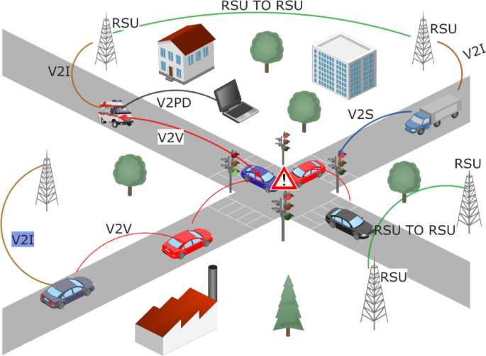
Consider a group of vehicles sharing information with RSUs stationed at the intersections of roads. The car devices can communicate with the roadside units using special communication technology. Every roadside unit in the network is located together with a server at the edge, where the deep learning models are installed. The fog servers are linked to the cloud servers using fast-wired connections. While the actual vehicle misbehavior prediction tasks are conducted on the fog servers, the deep learning models are developed on cloud servers. When data is transmitted by a vehicle, it is received by the nearest RSU. The data is then sent by the RSU to the edge server to check for any improper behavior. The network model depicted in Fig. 3 illustrates this process.
Fig. 3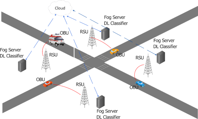
Proposed system network model.
By integrating fog computing into VANETs, the proposed framework can adapt to different environmental situations, including challenging weather conditions like rain, fog, or snow. In these scenarios, sensor data may become unreliable, delayed, or even partially lost, which can impact the quality of information gathered from vehicles.
Fog nodes, located nearer to the network’s edge, facilitate real-time data filtering, aggregation, and preprocessing, which improves the dependability of the input data before it is sent to the classification model. This local processing reduces the adverse effects of environmental disturbances.
Additionally, the deep learning model has been trained on a wide range of behavioral patterns that can represent both sensor malfunctions and unpredictable driving behaviors, some of which can be indirectly affected by weather. This setup enables the model to distinguish between erroneous sensor readings caused by environmental factors and deliberate malicious actions, thus ensuring strong detection performance in difficult operating conditions.
The cars could behave in a normal manner or exhibit several types of misbehavior. Misbehavior can be categorized into different faults or attacks. This study utilized data from the VeReMi Extension, which is a popular dataset for detecting misbehavior in vehicular networks40. This dataset includes a variety of kinds of misbehavior, including cyberattacks like Denial of Service (DoS) attacks, replay attacks, and their variations41, as well as errors relating to wrong location and velocity measurements. According to the behavior of the vehicle, action is taken.
Data preprocessingStructure of the dataset
There are 24-hour simulations in the VeReMi Extension dataset, one for each hour of the day from hour 0 to hour 23. Each simulation consists of one Ground Truth (GT) file comprising all the data that was received by the fog servers during that hour, combined with the original trace logs of each vehicle that traveled through the network during that hour. Send time, sender ID, sender pseudoID, message ID, and position-based information, such as location, velocity, acceleration, and direction, as well as the noise in each of these variables, are just a few of the fields that make up the data in these log files and the GT file of each simulation. The 24 GT files were utilized since the study focused on misbehavior detection at the level of fog servers.
Fig. 4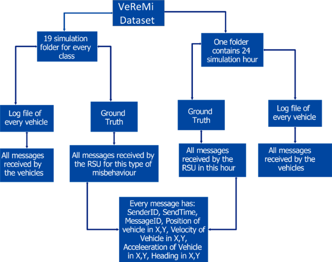
illustrates the full structure of the dataset.
Figure 4 Hierarchical structure and feature details of the VeReMi dataset.
Field selection and labeling
Sender ID, sender pseudoID, send time, two X and Y coordinate values of each position, velocity, acceleration, and direction, among other data fields provided in the GT file, are necessary for our investigation. The vehicle entries provided in the GT files do not have any misbehavior labels attached to them. The vehicle-wise log files for the relevant simulation hour provide this information. All the simulated hours’ GT files were studied. Then, it was chosen to select all the features and provide misbehavior labels from the log file names for each given vehicle to generate a simplified vehicle-wise dictionary that contained the labels and data required for each.
Sequence creation
Several experiments were conducted to choose the optimal sequence length. When larger sequence lengths (greater than 20) were tested, the number of generated sequences decreased substantially for several minority classes. As a result, some classes contained insufficient samples for effective training and evaluation, while others became severely underrepresented. This negatively affected class coverage and increased class imbalance within the generated sequence dataset.
Conversely, smaller sequence lengths were also examined. Although they increased the number of generated sequences, they significantly increased the computational cost and training time without providing a noticeable improvement in classification performance.
Based on these observations, a sequence length of 10 was selected as a practical compromise between preserving class representation, maintaining computational efficiency, and achieving strong classification performance.
The reduced vehicle data dictionary was used to produce several time sequences, each with ten data points. Label, send time, pseudoID, X and Y location coordinates, X and Y position noise coordinates, X and Y velocity coordinates, X and Y velocity noise coordinates, acceleration and heading coordinates, and their noise in the coordinates of X and Y. All are the variables that make up each data point. Sequences shorter than ten were not taken into consideration. Once all a vehicle’s time sequences have been created, they are added to the dictionary of misbehavior class as shown in Algorithm 1. Figure 5 shows the flow chart of the preprocessing of data.
Fig. 5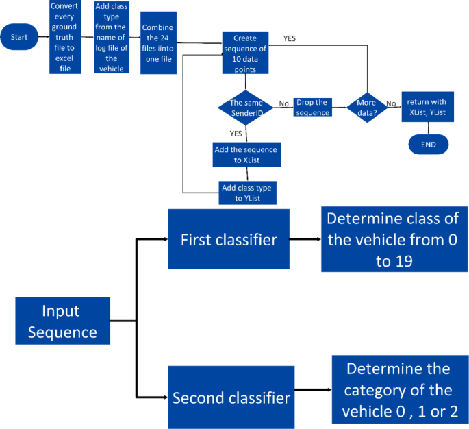
Flow chart of preprocessing.
Algorithm 1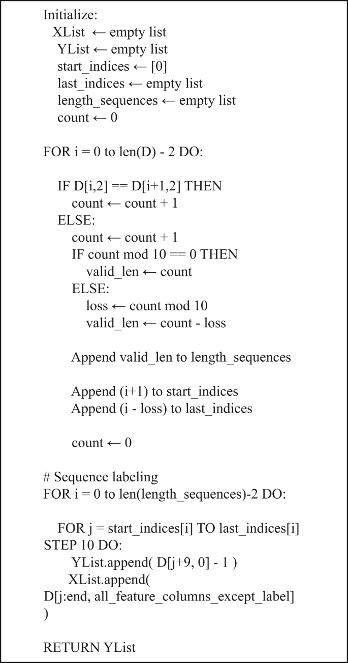 Misbehavior class selection
In this study on classification, the goal is to classify twenty different class types from the original VeReMi Extension dataset. As seen in Table 3, this contains one normal vehicle behavior type, nine fault kinds, and ten attack types. The number of generated sequences for each behavior class after sequence construction, illustrating the class distribution used throughout the experiments.
Table 3 Classes and their sequences.
The abnormal behaviors observed in the dataset are categorized into two separate groups: fault classes and attack classes, depending on the nature and purpose of the deviation.
Fault Classes indicate unintended, non-malicious irregularities that often arise from sensor failures or calibration mistakes. These faults impact both positional and velocity data:
a.
Positional faults: where a vehicle inaccurately reports its location with either constant or random discrepancies, either holding a steady position or changing it erratically.
b.
Velocity faults: where a vehicle alters its speed by introducing constant or random changes to its actual velocity, replicating unusual movement patterns.
Attack Classes consist of deliberate, malicious actions intended to disturb the network or deceive other nodes. These encompass:
a.
Denial of Service (DoS): overwhelming the network with an excessive number of messages, denying vehicle nodes the ability to access the infrastructure’s operational capabilities.
b.
Sybil Attacks: employing numerous fake identities (pseudoIDs) to exert inappropriate influence in the network. Due to the authenticity of the IDs, identifying such misconduct is challenging.
c.
Data Replay: retransmitting previously recorded legitimate data from another vehicle, complicating detection due to the utilization of authentic patterns.
d.
Disruptive Attacks: A variant of data replay where messages from several vehicles are randomly broadcast, leading to network congestion.
e.
Eventual Stop Attack: The vehicle halts its position and adjusts its velocity to zero, creating the illusion of an abrupt and unrealistic stop.
Table 4 presents the key differences between fault and attack classes.
Table 4 Comparison between fault and attack classes.Deep learning classifier
Deep learning imitates the human brain’s ability to assimilate data and develop patterns from it to make decisions, and it can learn from unstructured and unlabeled data. Deep learning models include Multi-Layer Perceptron (MLP), Convolutional Neural Network (CNN), Recurrent Neural Network (RNN), and Long Short-Term Memory (LSTM).
A CNN is a hierarchical system that applies a sliding filter with a defined width to the input of each convolutional layer. After each epoch, the sliding filter adjusts to capture new observations. The input may be one dimension (1D) or more. In the present investigation, we use 1D convolutional layers. A CNN consists of an input layer, many hidden layers, and an output layer. The hidden layers consist of convolutional layers followed by normalization, pooling, or fully connected layers.
LSTMs are a sort of RNN that retains sequential information. RNNs outperform ANNs on sequential data, but they also suffer from vanishing gradient issues. This impairs the network’s ability to remember information over long periods of time since any two critical events in the time series may occur with large gaps. LSTMs are designed to tackle the problem of disappearing gradients by being somewhat insensitive to the gap length. Because of their ability to recall values across arbitrary time intervals, LSTM networks are ideal for classification issues involving time series data.
Because of the time-series structure of vehicle data, CNN and LSTM are the ideal deep learning models. Furthermore, combining both techniques will be quite beneficial in maximizing their respective benefits. Thus, the CNN and LSTM models are used in this study to classify misbehavior in sequential vehicular data.
We describe here two alternative types of classifiers for classifying and detecting potential intrusions in the IoV network.
First classifier
It is a classifier in which the deep learning model predicts and classifies the input sequence as normal, one of the eight fault categories, or one of the eleven assault types determined.
Second classifier
It is a classifier in which the deep learning model predicts and classifies the input sequence as normal, fault, or attack type.
Training and testing
For all training of the deep learning models, “categorical_crossentropy” was chosen as the loss function as it is a multiclass classifier. The Adam optimizer is used with a learning rate of 0.0003. The dense layers are activated with the “softmax” activation function. Accuracy, precision, recall, and F1-score are defined in Eq. (1), Eq. (2), Eq. (3), and Eq. (4), respectively.
$$\text{Accuracy} = \frac{TN+TP}{TN+FP+FN+TP}$$
(1)
$$\text{Precision}= \frac{TP}{TP+FP}$$
(2)
$$\text{Recall}= \frac{TP}{TP+FN}$$
(3)
$${\text{F}}1_{\text{Score }}= 2* \frac{Precision*Recall}{Precision+Recall}$$
(4)