Lu+ optical frequency references with accuracy verified at the 19th digit

Experimental sequence

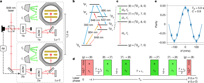
Each interrogation beginsonly after both ions have been subjected to Doppler cooling and prepared in the |g⟩ state with >99% probability using the conditional state preparation sequence described in ref. 53. Both ions are interrogated with the HA–HR sequence shown in Fig. 1d, with the parameters τL ≈ 4 ms, τ1 = τ2 ≈ 12 ms, and a total Ramsey time given by TR = 3(T + τ1 + τ2). Comparisons of the two independent frequency references are carried out by measuring the parity alternately for \(\phi =\pm \frac{{\rm{\pi }}}{2}\) and, after N interrogation cycles, steering \(\varPi \left(\frac{{\rm{\pi }}}{2}\right)-\varPi \left(-\frac{{\rm{\pi }}}{2}\right)\) to zero by updating δf. For the comparisons at the same 0.1 mT magnetic field, as is the case for all results shown in Fig. 2, the microwave drive frequencies f1 and f2 are identical for both ions and fixed throughout. For comparisons at different magnetic fields, as when evaluating the quadratic Zeeman coefficient αz, the microwave frequencies are necessarily different to compensate quadratic Zeeman shifts. The frequency difference δf is set by an acousto-optic modulator (AOM), labelled AOM 2a in Fig. 1a. Two auxiliary measurements are interleaved with the comparison servo: Rabi spectroscopy of the \(| g\rangle \leftrightarrow | 8\rangle \) optical transition to ensure the 848 nm clock laser is near resonance and measurement of the \({|}^{3}{D}_{1},6,\pm 1\rangle \) Zeeman splitting for each ion using microwave spectroscopy. The Zeeman splitting is used to infer the magnetic field, and feedback is applied to shim coils to compensate for any slow field drift, with further details in the Supplementary Information. HA–HR interrogation time is typically 87% of the total duty cycle, including the auxiliary measurements.

Magnetic field stability and servo

The short-term stability of the magnetic field is shown in Extended Data Fig. 2 (blue points). This was evaluated from a separate experiment measuring a Zeeman splitting with fast servo attack time. Over the range of Ramsey times of interest in this work (about 1–50 s), the magnetic field noise shows flicker instability of approximately 7 nT. During comparison measurements, the magnetic field is steered to the set point of B0 = 0.1 mT by a compensation coil with a typical servo attack time of tser ≈ 80 s using interleaved measurements of the \({|}^{3}{D}_{1},6,\pm 1\rangle \) Zeeman splitting. The orange points in Extended Data Fig. 2 show the field instability inferred from the in-loop measurements of the \({|}^{3}{D}_{1},6,\pm 1\rangle \) Zeeman splitting, which averages down ∝(tser/τ) for reasons explained in the Supplementary Information. The true instability of the magnetic field is limited by both projection noise and deadtime \(\propto {({t}_{{\rm{ser}}}/\tau )}^{1/2}\), which was verified in a test run using interleaved out-of-loop measurements of the \({|}^{3}{D}_{1},8,\pm 1\rangle \) Zeeman splitting (Extended Data Fig. 2, green points). This out-of-loop stability is taken as an upper bound on the magnetic-field instability with compensation engaged. The magnetic field contributes uncertainty through the quadratic Zeeman shift of \(\frac{\delta {\nu }_{\mathrm{QZ}}}{{\nu }_{0}}=2{\alpha }_{z}{B}_{0}\delta B(\tau )\approx 2\times 1{0}^{-19}\times {(\tau /{\rm{s}})}^{-1/2}\) beyond the servo attack time.

Detection and background gas collisions

To detect background collisions as much as possible and ensure the ions are sufficiently re-cooled before the next experiment cycle, we use the detection sequence shown in Extended Data Fig. 3a at the end of every Ramsey experiment. The intervals di represent adaptive Bayesian state detection54 by 646 nm fluorescence. If the ion is detected dark in the initial detection d0 after the Ramsey sequence, which is about 50% of events, then three attempts are made to shelve on the 848 nm clock transition and detect. The variable 848 nm clock pulse areas are tailored to maximize population transfer even for higher thermally occupied vibrational n states. The probability of at least one successful shelving is >99.5% for the expected thermal distribution accounting for ion heating during the Ramsey dark time TR. If the ion is not detected bright on any of d0…3, then it is assumed that a collision has occurred with sufficient energy transfer to significantly reduce either (1) the coupling on the 848 nm transition or (2) the 646 nm fluorescence rate. During clock comparison servo operation, if a collision is detected in this way on either Lu-1 or Lu-2, that interrogation cycle is considered invalid and repeated.

If a collision is detected (d0…3 all dark), the additional ending sequence shown in Extended Data Fig. 3a is applied. First, a repump pulse (350 nm, 622 nm and 895 nm) and another detection d4 is attempted. If bright, this is attributed to a lower-energy-transfer collision of type 1: sufficient to reduce efficiency of shelving on the clock transition but not detection. If dark, then the collision is of type 2: energetic enough to disrupt detection. In either case, a cycle of cooling and fluorescence detection with a high threshold, bi, is repeated until the ion is confirmed bright to ensure the ion is effectively cooled for the next experiment cycle. Extended Data Fig. 3b shows the probability of outcomes (1) and (2) as a function of TR from which we extract rates Γ(1) and Γ(2). To estimate the detectable collision rate Γ, we assume \({\varGamma }^{(1)}=\frac{1-{P}_{{\rm{d}}}}{2}\varGamma \) and Γ(2) = PdΓ, where Pd is the probability a collision interferes with bright detection, resulting in outcome (2). Of the lower energy transfer collisions at rate (1 − Pd)Γ, we assume half are not detected because the ion was in 3D1 at the end of the Ramsey experiment and half are detected as outcome (1). We infer the collision rates Γ = 1.9 × 10−3 s−1 for Lu-1 and 5.9 × 10−3 s−1 for Lu-2.

After the comparison measurement campaign, additional experiments were performed to estimate the collision rate without the complications introduced by Ramsey spectroscopy. The ions were prepared in the 1S0 ground state, and after a delay of 5 s, an attempt was made to reshelve and detect using a similar sequence as shown in Extended Data Fig. 3a. From the probability that all of multiple shelving attempts on the clock transition fail, we directly infer the detectable collision rates Γ = 2.9(3) × 10−3 s−1 for Lu-1 and 6.5(6) × 10−3 s−1 for Lu-2, in reasonable agreement with the rates inferred from the measurement campaign data.

Our extensive analysis of collision shifts in ion-based optical clocks is given in ref. 24. The collision shift is evaluated with respect to a Langevin collision rate ΓL, defined as the rate of collisions below a critical impact parameter that result in an inward-spiralling trajectory. We calculate the overestimate of the Langevin collision rate using eq. 31 of ref. 24 and with the cutoff velocity given by the 50% threshold of the Ramsey suppression factor as defined in section 2 of ref. 24. Using ω ≈ 1 MHz for Lu-1 and ω ≈ 500 kHz for Lu-2 yields ΓL = 1.3 × 10−3 s−1 and 2.1 × 10−3 s−1 for the respective Langevin rates, corresponding to 3.5 nPa and 5.8 nPa background pressures of molecular hydrogen at 300 K and consistent with pressure gauge readings. An inverted magnetron gauge on Lu-1 reads 4 nPa, and the ion pumps on both chambers read ‘low pressure’ (<13 nPa) at the limit of the sensitivity of the ion pump controllers. With κ = 1 in eq. 60 of ref. 24, we estimate collision shift bounds of 3.9 × 10−20 and 3.2 × 10−20 for Lu-1 and Lu-2, respectively.

Blackbody radiation

The differential dynamic polarizability, Δα(ω), for the 848-nm clock transition in 176Lu+ has been well characterized39,40. The BBR shift is given by

$$\frac{\delta {\nu }_{\mathrm{BBR}}}{{\nu }_{0}}=-4.90\times 1{0}^{-19}{\bar{T}}^{4}(1+1.77{\bar{T}}^{2}),$$

(2)

where \(\overline{T}\equiv T/{T}_{0}\) and T0 = 300 K. Over the practical temperature range of 270–330 K, the uncertainty contribution from Δα(ω) is well approximated by \(9.8\times 1{0}^{-20}{\bar{T}}^{4}\) (ref. 40). A detailed temperature assessment is given in the Supplementary Information in which we bound the minimum and maximum temperatures to [299.8, 303.2] K for Lu-1 and [299.6, 301.9] K for Lu-2.

Trap secular frequencies

The Lu-1 trap used in previous work16 had an unusually high heating rate, which has been resolved after replacing the ion trap with one of the same design53. Moreover, the helical resonators for both Lu-1 and Lu-2 were changed to reduce the RF-drive frequency ΩRF and obtain higher trap confinement without increased RF power. For 0.25 W of RF power at ΩRF = 2π × 9.4 MHz and 11.2 MHz, we obtain secular trapping frequencies of (207, 1,063, 1,134) kHz and (138, 492, 543) kHz for Lu-1 and Lu-2, respectively, in which the weakest confinement corresponds to the axial direction. The combined effect of reduced heating rates and the smaller Lamb–Dicke parameters resulting from the increased radial confinement means ion heating is no longer a significant limitation to the interrogation time. The simulated contrast loss shown in Fig. 2a is evaluated by averaging the final optical pulses over a thermal distribution of radial mode occupation accounting for the heating during the Ramsey time.

Thermal second-order Doppler

Thermal motion gives rise to an SODS given by

$$\frac{\delta {\nu }_{\mathrm{SODS}}}{{\nu }_{0}}=-\frac{\langle {v}^{2}\rangle }{2{c}^{2}}=-\frac{{k}_{{\rm{B}}}}{2m{c}^{2}}\sum _{i}({\kappa }_{i}{T}_{i}),$$

(3)

where Ti are the average temperatures during the Ramsey interrogation for the axial (i = 1) and radial (i = 2, 3) principal axes, respectively, and kB is Boltzmann’s constant. The geometry factor κ2 = κ3 ≈ 2 accounts for equal contributions from the secular motion and intrinsic micromotion for the two radial principal axes, which is valid when the confinement is predominantly ponderomotive55. Axial confinement is predominantly due to the static potential, and so only secular motion contributes (κ1 ≈ 1).

The initial temperatures and heating rates are determined by measuring the temperature immediately after Doppler cooling and after a fixed delay time. The axial temperature is measured by fitting the thermal dephasing of Rabi flopping on the 804 nm E2 transition. Although the 804 nm laser wave vector is at 45° with respect to the ion trap axis and has a projection onto all principal axes, the radial modes have sufficiently low thermal occupation \(\overline{n}\) and a small Lamb–Dicke parameter η that they contribute negligibly to the thermal dephasing. From the weighted mean of three measurements over the course of the campaign, we find the initial temperatures T1,0 = 190.5(5.9) μK for Lu-1 and 189.6(4.7) μK for Lu-2 and heating rates \(\frac{{\rm{d}}{T}_{1}}{{\rm{d}}t}=73(14)\,\mathrm{\mu K}\,{{\rm{s}}}^{-1}\) for Lu-1 and 119(17) μK s−1 for Lu-2 (Extended Data Fig. 5). The average temperature during the Ramsey experiment for each mode is given by \({T}_{i}={T}_{i,0}+\frac{{\rm{d}}{T}_{i}}{{\rm{d}}t}\frac{{T}_{{\rm{R}}}}{2}\).

The radial temperatures are measured by spectroscopy on the secular-motion sidebands using the 804 nm E2 transition. The average thermal occupation \(\overline{n}\) of one of the radial modes is extracted from the ratio of population transferred on the red and blue sidebands56:

$$\frac{{P}_{\mathrm{red}}(t)}{{P}_{\mathrm{blue}}(t)}=\frac{\bar{n}}{\bar{n}+1}.$$

(4)

For both traps, the initial \(\overline{n}\) measurements on both radial modes are consistent with the temperature 150(30) μK, which is also consistent with the initial axial temperatures to within statistical uncertainty and corresponds to approximately three times the Doppler cooling limit. The sideband ratio method is most sensitive for low \(\overline{n}\), so for measuring the radial heating rates, we first apply Zeeman-degenerate Raman sideband cooling57 to prepare in the motional ground state and then measure the sideband ratio after some delay. Extended Data Fig. 6 shows the results of radial heating measurements in both chambers, which yield heating rates \(\left[\frac{{\rm{d}}{T}_{2}}{{\rm{d}}t},\frac{{\rm{d}}{T}_{3}}{{\rm{d}}t}\right]=[110(15),29.1(2.9)]\,\mathrm{\mu K}\,{{\rm{s}}}^{-1}\) for Lu-1 and [85.5(5.5), 70.4(5.5)] μK s−1 for Lu-2.

Equation (3) is the SODS for a thermal state in the high-temperature limit, \({\bar{n}}_{i}\approx \frac{{k}_{{\rm{B}}}{T}_{i}}{\hbar {\omega }_{i}}\), and does not account for the zero-point fluctuations for the quantum ground state for both secular and micromotion58,59, which contribute additional SODS of \(-\sum _{i}{\kappa }_{i}\left(\frac{\hbar {\omega }_{i}}{4m{c}^{2}}\right)\). This term contributes only a 6% correction to the total SODS for Lu-1 but has been included for completeness.

We estimate the total SODS for a Ramsey time TR as follows:

$$\begin{array}{c}(\mathrm{Lu}\text{-1})\,\frac{\delta {\nu }_{\mathrm{SODS}}}{{\nu }_{0}}=-2.4(2)\times 1{0}^{-19}+{T}_{{\rm{R}}}[-4.6(4)\times 1{0}^{-20}\,{{\rm{s}}}^{-1}],\\ (\mathrm{Lu}\text{-2})\frac{\delta {\nu }_{\mathrm{SODS}}}{{\nu }_{0}}=-2.4(2)\times 1{0}^{-19}+{T}_{{\rm{R}}}[-5.7(3)\times 1{0}^{-20}\,{{\rm{s}}}^{-1}].\end{array}$$

Excess micromotion

The micromotion shift has two components: an SODS due to oscillatory motion and the a.c. Stark shift due to the RF electric field. Owing to the very low differential polarizability of the clock transition, the a.c. Stark contribution is more than two orders of magnitude smaller than the SODS component and therefore negligible. The micromotion amplitude is evaluated using phase-modulated sideband spectroscopy on the 804-nm E2 clock transition22. The excess micromotion (EMM) SODS is given by

$$\frac{\delta {\nu }_{\mathrm{EMM}}}{{\nu }_{0}}=-{\left(\frac{{\varOmega }_{\mathrm{RF}}}{2c{k}_{804}}\right)}^{2}|\beta {|}^{2},$$

(5)

where k804 is the wavenumber of the 804-nm clock transition, and β is the modulation depth. As phase-modulated sideband spectroscopy is sensitive to the phase of the micromotion, we distinguish between two quadrature components β = βm + iβp, where βm is the excess micromotion due to displacement by stray fields, and βp is due to a phase shift between RF electrodes, which we are not able to compensate. Intrinsic micromotion is accounted for separately with the thermal SODS.

Following the procedure described in ref. 22, we measure the modulation depth in three orthogonal directions to evaluate \({\beta }_{{\rm{m}}}^{2}=\sum _{i}{\beta }_{{\rm{m}},i}^{2}\). The results of all measurements of βm,i taken for both ion traps are shown in Extended Data Fig. 4a,b, in which the open circles are measured before compensating for the d.c. stray field and closed circles immediately after. To estimate the EMM shift for each comparison measurement, we linearly interpolate the βm,i measurements, assuming linear growth of the d.c. stray field between measurements. Extended Data Fig. 4c shows the EMM shifts evaluated from the time average of \({\beta }_{{\rm{m}}}^{2}\) over each comparison interval. We estimate an average relative shift of −1.6(1.3) × 10−20 for Lu-1 and −1.4(0.4) × 10−20 for Lu-2.

As reported in ref. 22, βp is negligibly small for Lu-1. For Lu-2, the three orthogonal components of βp are measured to be [2.22(13), 1.43(12), 1.92(13)] × 10−2, corresponding to an EMM shift of −2.42(19) × 10−19. βp was remeasured at the end of the campaign and found to be in statistical agreement with the original measurement.

a.c. Zeeman, RF

Time-varying magnetic fields give rise to an a.c. Zeeman shift, with the dominant contributions coming from currents in the electrodes driven by the RF-trapping potential. The contribution depends on the component of the RF magnetic field perpendicular to the applied d.c. field60. The clock shift given by

$$\delta {\nu }_{\mathrm{RF}}={\alpha }_{\perp }\langle {B}_{\perp }^{2}\rangle ,$$

(6)

where \(\sqrt{\langle {B}_{\perp }^{2}\rangle }\) is the root-mean-square RF magnetic field amplitude perpendicular to the d.c. field and α⊥ = 0.20 mHz μT−2 is the sensitivity coefficient after 3D1 hyperfine averaging60.

Although in previous work B⊥ was measured using an Autler–Townes splitting on the Ba+ clock transition41, here we use an Autler–Townes splitting on the Lu+3D2 |6, 0⟩ to |5, 0⟩ microwave transition. The 3D2 F = 5 Landé g-factor, g5 = −0.38575750(19) (ref. 53), is the largest of all 3D1 and 3D2 F manifolds, and for ΩRF ≈ 2π × 10 MHz, the linear Zeeman splitting can be brought into resonance with ΩRF at experimentally accessible magnetic fields of B ≲ 2 mT.

The experimental measurement procedure is as follows. Neodymium permanent magnets are used to bias the magnetic field to the required 1.7 mT for Lu-1 and 2.0 mT for Lu-2. Three pairs of coils are used to fine-tune the magnetic field amplitude and optimize the orientation for the \({|}^{3}{D}_{1},7,0\rangle \) state preparation by aligning to a π-polarized 646-nm laser. This ensures the d.c. magnetic field is aligned in the same direction as during the comparison measurements. From \({|}^{3}{D}_{1},7,0\rangle \), we transfer sequentially to the \({|}^{3}{D}_{1},8,0\rangle \) state using a microwave π pulse and then the \({|}^{3}{D}_{2},6,0\rangle \) state using an 804-nm–848-nm Raman pair. We observe the Autler–Townes splitting by interrogating the \({|}^{3}{D}_{2}\,| 6,0\rangle \) to |5, 0⟩ microwave transition with a π pulse for a range of detunings, after which the remaining \({|}^{3}{D}_{2},6,0\rangle \) population is reshelved to \({|}^{3}{D}_{1}\rangle \) by Raman transfer for detection.

Following the treatment in ref. 60, the effective Hamiltonian in the rotating wave approximation describing the microwave interrogation is

$$H=\frac{\hbar }{2}\left(\begin{array}{cccc}-2{\varDelta }_{{\rm{M}}} & {\varOmega }_{M} & 0 & 0\\ {\varOmega }_{M} & 0 & {\varOmega }_{B} & {\varOmega }_{B}\\ 0 & {\varOmega }_{B} & 2{\varDelta }_{1} & 0\\ 0 & {\varOmega }_{B} & 0 & -2{\varDelta }_{-1}\end{array}\right),$$

(7)

where ΩM is the microwave coupling, ΔM is the microwave detuning, \({\varOmega }_{B}=\frac{1}{\hbar }\frac{\sqrt{15}}{2}{g}_{5}{\mu }_{B}{B}_{\perp }\) is the coupling between \({|}^{3}{D}_{2},5,0\rangle \) and |5, ±1⟩ states due to the transverse oscillating magnetic field at frequency ΩRF, and

$${\varDelta }_{\pm 1}={\varOmega }_{{\rm{R}}{\rm{F}}}\pm {\omega }_{\pm 1}={\varOmega }_{{\rm{R}}{\rm{F}}}+{g}_{5}{\mu }_{B}B/\hbar \pm 2\pi \times \varDelta \alpha {B}^{2}$$

(8)

is the detuning of the RF field from the |5, 0⟩ to |5, ±1⟩ Zeeman splittings, ω±1. Degeneracy of ω±1 is lifted by the differential quadratic Zeeman shift for which Δα ≈ 1.23 kHz mT−2.

Extended Data Fig. 7a shows the simulated spectrum of the Autler–Townes splittings for the operating parameters of Lu-1 and ΩB =2π × 3 kHz. For both Lu-1 and Lu-2, several spectra were taken at a fixed magnetic field in the vicinity of the Autler–Townes splitting, of which three from Lu-1 are shown in Extended Data Fig. 7b–d. We fit the measured data to simulated spectra to obtain ΩB. Taking the mean of the ΩB fit values, with the standard deviation of fit values as the uncertainty, we find \(\sqrt{\langle {B}_{\perp }^{2}\rangle }\) to be 0.220(5) μT and 0.303(4) μT for Lu-1 and Lu-2, respectively. The RF-drive voltage to the trap is monitored over the campaign and for both Lu-1 and Lu-2 varied by less than 0.5%.

a.c. Zeeman, microwave

When applying the microwave fields during the Ramsey sequence for hyperfine averaging, there is a probe-induced shift because of the σ± polarization components off-resonantly coupling to m = ±1 Zeeman states. Evaluation of this shift is discussed in detail in the supplementary material of ref. 16. The total microwave a.c. Zeeman shift is given by

$$\delta {\nu }_{\mu }=\frac{({\varDelta }_{1,7}+{\varDelta }_{1,8}){\tau }_{1}+({\varDelta }_{2,6}+{\varDelta }_{2,7}){\tau }_{2}}{{T}_{{\rm{R}}}},$$

(9)

where Δk,F is the shift of |F, m = 0⟩ when microwave coupling Ωk is on. The microwave field polarizations are characterized by measuring the π times τkq for the field k and polarization q, at fixed microwave power, from which the shifts Δk,F are evaluated as

$$\begin{array}{c}{\varDelta }_{1,8}=-\frac{7}{9}\frac{{\varOmega }_{1}^{2}}{4{\omega }_{7}}\left[{\left(\frac{{\tau }_{10}}{{\tau }_{1+}}\right)}^{2}-{\left(\frac{{\tau }_{10}}{{\tau }_{1-}}\right)}^{2}\right],\\ {\varDelta }_{1,7}=\frac{{\varOmega }_{1}^{2}}{4{\omega }_{8}}\left[{\left(\frac{{\tau }_{10}}{{\tau }_{1+}}\right)}^{2}-{\left(\frac{{\tau }_{10}}{{\tau }_{1-}}\right)}^{2}\right],\\ {\varDelta }_{2,7}=\frac{{\varOmega }_{2}^{2}}{4{\omega }_{6}}\left[{\left(\frac{{\tau }_{20}}{{\tau }_{2+}}\right)}^{2}-{\left(\frac{{\tau }_{20}}{{\tau }_{2-}}\right)}^{2}\right],\\ {\varDelta }_{2,6}=\frac{4}{3}\frac{{\varOmega }_{2}^{2}}{4{\omega }_{7}}\left[{\left(\frac{{\tau }_{20}}{{\tau }_{2+}}\right)}^{2}-{\left(\frac{{\tau }_{20}}{{\tau }_{2-}}\right)}^{2}\right],\end{array}$$

where ωF > 0 is the Zeeman splitting for the hyperfine level F.

This shift is suppressed by ensuring τk ≪ TR, balancing the circular polarization components (τk+ ≈ τk−), and maximizing the π coupling (τk0 ≪ τk±). All microwave horns are mounted on rotation mounts and are tuned, through a combination of translation and rotation, to the condition τk+ ≈ τk− as much as possible at the start of the campaign. All τkq were characterized at three points in the campaign, and the evaluated clock shifts were consistently below 1 × 10−20.

Quadrupole shift

The hyperfine-averaged residual quadrupole moment has been reported as \(\widetilde{\varTheta }=-2.54(0.25)\times 1{0}^{-4}\,e{a}_{0}^{2}\) (ref. 42), which has been independently confirmed by an alternate method23. The residual quadrupole shift, \(\delta {\widetilde{\nu }}_{Q}\), is evaluated by measuring the quadrupole shift, δνQ,1, on the 3D1 |7, 0⟩ to |8, 0⟩ microwave clock transition, which are related by

$$\delta {\widetilde{\nu }}_{Q}=\frac{\widetilde{\varTheta }}{\frac{8}{5}\varTheta {(}^{3}{D}_{1})}\delta {\nu }_{Q,1},$$

(10)

where \(\varTheta {(}^{3}{D}_{1})=0.63862(74)\,e{a}_{0}^{2}\) (ref. 61). We measure the microwave transition frequencies for both traps by microwave Ramsey spectroscopy with a 10 s interrogation time. The quadrupole shifts δνQ,1 are inferred using the unperturbed microwave frequencies23 and accounting for the second-order Zeeman shifts. The residual quadrupole shifts on Lu-1 and Lu-2 are evaluated to be 3.3(3) × 10−20 and 1.35(14) × 10−19, respectively. Given the accuracy of the measured unperturbed microwave frequencies23, the quadrupole shift may be easily suppressed further by setting the magnetic field angle so as to null the microwave quadrupole shifts as much as is required.

Microwave coupling errors

Incorrect microwave pulse areas due to uncertainty in the respective couplings give rise to timing errors in HA–HR spectroscopy. As derived in the supplementary material of ref. 16, the shifts due to microwave coupling errors are bound by

$$\delta {\nu }_{k}\approx -\frac{1}{{T}_{{\rm{R}}}}\left({\left(\frac{{\varDelta }_{k}{\tau }_{k}}{\pi }\right)}^{2}+{\left(\frac{\pi {q}_{k}}{2}\right)}^{2}\right),$$

(11)

where Δk is the microwave detuning, τk is the microwave π pulse duration, and qk is the fractional error in the microwave coupling for the k = 1, 2 microwave transitions.

These shifts are suppressed for Ramsey times TR ≫ τL, τk, as is the case for the comparison experiments reported here. The magnetic field was actively steered to a fixed value in both chambers so the microwave detunings Δk are stable and known precisely from the quadrupole shift assessment. The microwave couplings were measured at the beginning, middle and end of the campaign with about 0.2% measurement precision and found to deviate by less than 0.5%, with the exception of Ω2 on Lu-2, which drifted by 1.5% from the beginning to the end of the campaign. Extended Data Fig. 8, for example, shows this shift evaluated for the worst case of q2 = 0.015 as a function of the detuning Δ2. Although the Δk are precisely known at the <10 mHz level, which, in principle, allows for a more accurate estimation of this shift, we take a conservative approach and use the full width of the bounding envelope, given by the second term in equation (11), as the uncertainty.

a.c. Stark

For an optical π time of \({\tau }_{{\rm{L}}}=\frac{{\rm{\pi }}}{{\varOmega }_{{\rm{L}}}}=4\,\mathrm{ms}\), the a.c. Stark shift on the |g⟩ to |8⟩ optical transition when interrogating with the 848-nm laser is approximately ΔS = 2π × 25 Hz. In the absence of additional effects, both the HR37 sequence, Extended Data Fig. 9a, which was used in previous work16, and the time-reversed HR sequence, Extended Data Fig. 9b, which is used in this work, equivalently suppress the resulting clock shift to \(\frac{2}{{\rm{\pi }}{T}_{{\rm{R}}}}{\left(\frac{\varDelta }{{\varOmega }_{{\rm{L}}}}\right)}^{3}\), in Hz, where Δ = ΔSP − ΔS is the error in the frequency step, ΔSP, applied during the optical interrogation pulses. To set the laser frequency step, ΔSP, the a.c. Stark shift was measured to better than 1% for both Lu-1 and Lu-2 at the start of the campaign by interleaved self-comparison of Rabi and HR spectroscopy. The value of the ΔSP was fixed throughout the campaign, and we bound the uncertainty in Δ to 2% of |ΔS| for Lu-1 and 5% of |ΔS| for Lu-2 based on the maximum observed variation in the optical couplings, which were measured at the beginning, middle and end of the campaign with measurement precision of about 0.2%.

When including the effects of ion heating, HR schemes present a weak linear dependence on Δ (ref. 62). This linear dependence is evaluated by simulation with the results for the typical operating parameters of Lu-2 shown in Extended Data Fig. 9c. It is noted that the linear slope has the opposite sign for HR and HR reverse schemes, and that a hybrid error signal constructed by averaging the two schemes cancels the thermal effect, restoring the cubic dependence on Δ. The idea of combining sequences to generate a more robust error signal is similar to modified HR63 and generalized HR64, but unlike those schemes for which ion heating results in either an offset or increased sensitivity compared with the basic HR scheme62, this simple hybrid combination of HR and HR reverse heavily suppresses the linear dependence on ion heating, at least in the regime τL ≪ TR, in which heating during the optical pulse is negligible compared with during the dark time TR.

For the experiments reported here, the shift was already sufficiently small that only HR reverse was used. From the measured radial heating rates, uncertainty in Δ and the linear dependence determined from simulation, we estimate a total uncertainty from the a.c. Stark effect to be 3.8 × 10−21 for Lu-1 and 2.5 × 10−20 for Lu-2 for TR = 5 s.

a.c. Quadrupole, RF

The oscillating RF quadrupole field couples off-resonantly to hyperfine transitions giving rise to an a.c. quadrupole shift that is not cancelled by hyperfine averaging65. We estimate this shift by assuming an ideal linear Paul trap with RF potential of the form Φ(x, y, z) = ϵ(x2 − y2) in the principal-axis frame, where the electric field gradient \({\epsilon }=\frac{m{\varOmega }_{\mathrm{RF}}{\omega }_{{\rm{r}}}}{e\sqrt{2}}\) is determined by the radial pseudo-potential confinement frequency ωr ≈ 2π × 1,100 kHz for Lu-1 and 510 kHz for Lu-2. The magnetic field in both chambers is aligned to approximately 33(3)° with respect to the ion trap axis (z). Under these conditions, we evaluate65 a relative clock shift of the HA frequency of −2.0 × 10−21 for Lu-1 and −5.7 × 10−22 for Lu-2.

Differential AOM chirp

As shown schematically in Fig. 1a, the differential path length is actively stabilized with reference to retroreflecting mirrors below the respective experimental chambers that are near the table surface and approximately 20 cm below the trapped ions. The differential phase stability is characterized by out-of-loop measurement of the optical phase with the clock beams directed to a common beam splitter instead of the ions, requiring approximately 2 m of additional unstabilized optical path length. When simultaneously switching on AOMs 1a and 2a, as for the Ramsey pulses in the comparison interrogation sequence, a differential phase chirp is induced by the lock circuitry as shown in Extended Data Fig. 10a. This is well modelled by a damped harmonic oscillation with the fit parameters shown in Extended Data Fig. 10a. By straightforward extension of the analysis given in ref. 66, we evaluate a −4.8(8) × 10−21 systematic shift to the difference frequency between Lu-1 and Lu-2 for TR = 5 s.

First-order Doppler

We consider two sources of first-order Doppler shift (FODS): drift of the ion with respect to the trap along the clock probe (vertical) direction and differential drifts of the optical phase.

The measured micromotion modulation depth βm,3 can be directly related to the displacement of the ion from the trap RF null along the clock interrogation direction22. For small modulation depth, the relationship is linear with scale factors of approximately 0.77 μm/βm,3 for Lu-1 and 2.0 μm/βm,3 for Lu-2. Extended Data Fig. 4d shows the evaluated FODS shift for each comparison measurement, where the average velocity is estimated from the inferred displacement between the EMM measurements. The weighted FODS for the entire campaign is estimated to be 2.4(3.5) × 10−23 for Lu-1, −0.3(2.0) × 10−22 for Lu-2 and 0.5(2.0) × 10−22 for the difference.

Using the same measurement setup as for AOM chirp, we measure the out-of-loop differential phase for long durations for which we observed an instability asymptote of 3.0 × 10−16 (τ/s)−1 as shown in Extended Data Fig. 10b (blue). For typical servo operation at 87% interrogation duty cycle, we evaluate a contribution of 2.0 × 10−17 (τ/s)−1/2 (orange). This is well below the comparison instability on all timescales. When operating as a single clock, the path length is actively stabilized from the laser to reference mirror instead of differentially between chambers, but can be expected to contribute at the same level or lower because of the shorter unstabilized path.

RF synthesis

The RF synthesizers used for the AOMs are based on the AD9912 chip and have approximately 7 μHz resolution. This contributes about 1 × 10−20 fractional uncertainty, half of the minimum step size, to the comparison servo. The synthesized microwave frequencies, f1 and f2, were identical and generated from the same sources for Lu-1 and Lu-2, set to the nearest 1 mHz. All synthesizers are referenced to a common hydrogen maser, which is calibrated to ≲2 × 10−15 at the start of the measurement campaign67. For the comparison measurement, any error in maser accuracy is common mode and contributes no uncertainty to the difference.

However, we note that when realizing a Lu+ standard using HA–HR spectroscopy as \({\nu }_{0}={f}_{{\rm{L}}}+\frac{1}{3}(2{f}_{1}+{f}_{2})\), the accuracy of the synthesized microwaves fk is also not a limitation to optical clock accuracy because the servo action steers the laser to compensate any errors in the microwave fields such that this specific linear combination of the fields is the HA frequency. The HA–HR servo is sensitive to the instability of both the laser and microwave fields at the same level, in Hz. In practice, this places a more relaxed requirement on the microwaves as compared with the laser; for example, for a laser with fractional instability \(\frac{\delta {f}_{{\rm{L}}}}{{f}_{{\rm{L}}}}\approx 1{0}^{-16}\), the microwaves need only a fractional stability better than \(\frac{\delta {f}_{k}}{{f}_{k}}\lesssim \frac{\delta {f}_{{\rm{L}}}}{{f}_{k}} \sim 1{0}^{-12}\) to not limit the clock instability.

Gravitational redshift

The differential redshift between the ions is given by \(\frac{g\delta h}{{c}^{2}}\), where g ≈ 9.776 m s−2 is the local gravitational acceleration and δh = h1 − h2 is the height difference of the ions. We measure the heights of the ions relative to a laser levelling assembly fixed to the optical table, which is precisely aligned to each ion by the same imaging optics used for state detection. We determine the ion heights h1 = 7.44(10) mm and h2 = 11.41(10) mm. Measurements of the table levelling by a precision spirit level with 0.02 mm m−1 resolution are limited by the table surface flatness but bound the table tilt to <0.2 mm m−1. The ion traps are separated by 1.2 m, and table levelling contributes the dominant uncertainty of 240 μm. The height difference of the ions is evaluated to be δh = −3.97(27) mm, corresponding to a −4.31(29) × 10−19 differential shift.

Clock stability

The stability of a single-ion optical clock is quantum-projection-noise limited at the longest achievable interrogation time, which is set by either the optical coherence of the local oscillator or the atomic coherence, whichever is shorter. State-of-the-art cavity-stabilized lasers reach fractional instabilities in the low 10−17 at 1 s (refs. 28,33) and have enabled demonstrated single-ion clock instabilities as low as 3.5 × 10−16 (τ/s)−1/2 (ref. 12). Although our laboratory lacks a local oscillator of this quality with which to challenge ion clock stability at this level directly, our comparison does probe the limits set by atomic coherence, allowing us to infer the technical limits to interrogation time independent of any clock laser. Comparison of two references by correlation spectroscopy carries a factor of √2 higher instability than a comparison of independent clocks, and a factor of 2 higher than a single standalone clock, for equal interrogation time. Insofar as the present comparison is limited by uncorrelated magnetic field noise, these systems, when combined with state-of-the-art laser stabilization, would support a single-clock instability of about 2.4 × 10−16 (τ/s)−1/2. Because the 3D1 lifetime imposes no practical limit, substantially longer interrogation times remain possible, contingent on overcoming magnetic field noise, ion trap heating and background gas collisions. Reducing the d.c. magnetic field lowers the linear sensitivity to field noise at the cost of smaller Zeeman splittings; nevertheless, operation at 25 μT is achievable with modest changes to our laser configuration. By our assessment, this would permit interrogation times up to 30 s in the present system. Even longer coherence times can be anticipated with the use of magnetic shielding and cryogenics, albeit at the cost of increased experimental complexity.