
To verify that the intended magnetic anisotropies were successfully imprinted during layer growth, the integral magnetization of both sensor designs was measured using an inductive BH-loop tracer. Figure 4a and b show the magnetization loops for the scissor-like and parallel-and-canted configurations, respectively. The combined magnetic easy axis and magnetic hard axis responses of the magnetic stack are shown in blue and red. For each measurement direction, the magnetization signal is measured parallel to the applied field and perpendicular to it, by switching by switching the orientation of the pick-up coil relative to the applied field and sample orientation. The component parallel to the applied field, corresponding to a cosine projection of the magnetization vector, is plotted as solid lines, while the perpendicular sine component is represented by dashed lines. This decomposition allows investigation of the underlying magnetization reversal process. In the case of reversible coherent rotation, the magnetization rotates continuously as a rigid vector, so that \(\:M\:\left|\right|\:H\) and \(\:M\perp\:H\) trace smooth, hysteresis-free curves. In contrast, reversal mediated by domain nucleation and domain-wall motion is irreversible and typically displays a finite hysteresis. In particular, measuring different courses of the transverse component along the hard axis is expected. For a single macrospin like behavior undergoing coherent magnetic rotation, the transverse magnetization reaches a maximum at remanence, whereas for a multi-domain state or related non macrospin behavior, the contributions from oppositely oriented domains may compensate, resulting in a reduced net transverse magnetization21,22. The effective anisotropy directions of each magnetic stack were determined by identifying the effective hard axis direction. These measurements reveal that the imprinted anisotropies during deposition exhibit slight angular offsets with respect to the intended directions for both sensor designs. For the scissor-like configuration, the effective anisotropy directions are rotated by 10° relative to the delay line. For the parallel-and-canted sensor, the extracted angle amounts to 14°, instead of the targeted 10°. These deviations in the direction of anisotropy likely arise from the interplay of unidirectional exchange-bias and stress-induced anisotropy16. Moreover, a non-collinear, tilted alignment of unidirectional anisotropy may occur in exchange-biased samples, including top-pinned MnIr-based layers23,24. In addition, minor temporal changes in the magnetic properties due to training effects of the exchange-bias may contribute to the observed offsets25. Also, the effective anisotropy directions of the individual layers within the scissor stack can be resolved. When the applied field is aligned parallel to the effective easy axis of an individual layer, the sine component vanishes, since magnetization reversal occurs just along the anisotropy direction, leaving no transverse magnetization contribution. The resulting alignments of the effective anisotropy directions \(\:{K}_{\text{e}\text{f}\text{f}}\) of the individual layers are displayed in Fig. 4c and d, respectively.
Fig. 4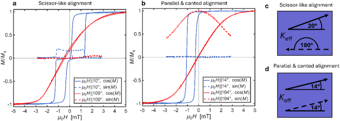
Hysteresis loops measured with a BH-loop tracer for (a) scissor-like alignment and (b) parallel & canted alignment. The blue curves correspond to the combined easy axis of the full stack and the red curves to the hard axis. The signal is divided in cosine (full line) and sine (dashed line) fraction of the magnetization. (c) Shows the deduced anisotropy directions \(\:\rm{K}_{eff}\) aligned along 20° and 180° for the two magnetic layer stacks for the scissor-like configuration. (d) For the parallel & canted configuration the effective anisotropy direction is aligned at 14°.
In Fig. 4a two well-separated hysteresis loops are observed (blue full curve), when a magnetic field is applied along 10°, the direction of the combined easy axis. This phenomenon is due to the presence of two exchange-biased magnetic layers whose effective anisotropies point in nearly opposite directions for the scissor-like design. At remanence, the loop exhibits a finite sine component of the magnetization (dashed line). While the applied field is aligned along the combined easy axis at 10°, the individual layer easy axes are oriented at 20° and 180°. For low magnetic fields, the magnetization aligns collinearly with the respective \(\:\rm{K}_{eff}\) of each layer. This results in a signal with twice the amplitude of the sine component of \(\:M\), arising from the perpendicular contributions of both layers. When the field reaches ± 1.5 mT, the magnetization of one layer switches, leading to cancellation of the sine components. Along the hard axis (\(\:H\) || 100°), a finite remanent magnetization exists and the magnetizations of the two layers rotate coherently22. The absence of a net transverse magnetization component in the corresponding dashed curve indicates that the two layers undergo coherent rotation in opposite directions, consistent with the intended scissor state.
In Fig. 4b, the parallel-and-canted sensor exhibits a single hysteresis loop along easy axis, characteristic for single exchange-biased magnetic layers. The loop is shifted to approximately − 0.6 mT. The perpendicular magnetization component vanishes at the effective hard axis angle (blue dashed curve), while a perpendicular field orientation (red dashed curve) produces the maximum response. The latter indicates that the magnetizations in both layers undergo coherent rotation in the same direction22 and suggests a single-domain magnetic state during magnetization-reversal for magnetic field applied along (\(\:H\) || 104°). Additional investigations of the magnetic domain configurations by large field-of-view magneto-optical Kerr effect (MOKE) microscopy26 are provided in the Supplementary Information.
Figure 5 summarizes the readout characteristics of the SAW magnetic field sensors, excited with 0 dBm. Figure 5a–c refer to the scissor-like alignment, while 4d–f show the results for the parallel-and-canted alignment. Figure 5a and d show the magnetic sensitivity when an AC magnetic field is applied at a perpendicular angle (90°) to the direction of SAW propagation, with a peak-to-peak field of 10 µT at 10 Hz. For the scissor-like alignment, the sensitivity at zero magnetic field amounts to (488 ± 10) °/mT. The sensitivity can be further enhanced, visible by the two distinct maxima at approximately 0.17 mT with 562 °/mT and 0.96 mT with 739 °/mT. In contrast, the parallel-and-canted configuration exhibits higher sensitivity maxima at 0.33 mT with 800 °/mT and 1.05 mT with 1006 °/mT, while the zero-field sensitivity is comparable at (490 ± 10) °/mT. Since none of the sensitivity maxima occur exactly at \(\:{\mu\:}_{0}H\) = 0 mT, the ideal magnetization states sketched in Fig. 3b and c are not fully achieved, which is consistent with the angular offsets extracted from the BH-loop tracer measurements. Because of the coherent rotation of magnetization, only a very small hysteresis is visible in the insets of the sensitivity curves.
Fig. 5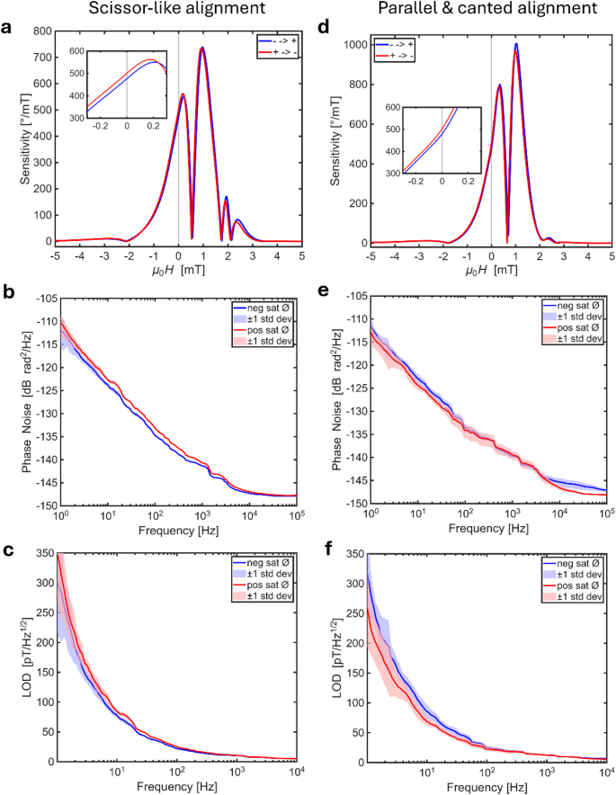
Electrical sensor characterization for different magnetic alignments. Blue and red curves correspond to measurements after negative and positive field saturation, respectively. All measurements were taken at 0 dBm. Plots a–c) show the scissor-like alignment, while plots d–f) show the parallel-and-canted alignment. a, d) Sensitivity as a function of applied field, with an inset highlighting the range ± 0.3 mT. b, e) Phase noise measured as an average over nine runs, with shaded areas indicating ± 1 standard deviation. c, f) Resulting LOD calculated from the sensitivity and phase noise data.
Figure 5b and e show the phase noise spectra of the sensors. Nine individual measurements were performed each after saturating the sensors in positive and negative magnetic field directions. From these data, an average phase noise and the corresponding standard deviation were calculated. The final noise measurements were carried out without any externally applied magnetic bias field. The phase noise spectrum exhibits the characteristic 1/f frequency dependence at offset frequencies up to 104 Hz, above which the frequency-independent thermal noise floor becomes dominant27. At a frequency of 10 Hz, the phase noise ranges between − 122 dBrad²/Hz and − 124 dBrad²/Hz for both sensor concepts. These values are approximately 5–7 dB lower than those reported for SAW sensors with antiparallel exchange-bias published by Schell et al.13. The lower noise level is consistent with the reduced sensitivity of the present sensors27. Since phase noise scales with sensitivity, the higher sensitivity reported by Schell et al.13 corresponds to a higher noise level of their sensor. It is also advantageous that no external bias field is applied during the noise measurement, as the bias field generation might add further noise. The generally low phase noise can be attributed to the domain state stabilized by the exchange-bias, which reduces the phase noise by about 7 dB compared to a multidomain thin film13,16. Only a small difference between the phase noise spectra measured after positive and negative saturation is observed, indicating only slightly different magnetic configurations. This observation is consistent with the remaining minor hysteresis seen in both the BH-loop tracer measurements and the sensitivity curves.
Figure 5c and f present the calculated LOD, obtained by dividing the phase noise by the sensitivity. For the scissor-like alignment, a LOD of (77 ± 4) pT/Hz1/2 after negative saturation and (84 ± 3) pT/Hz1/2 after positive saturation is achieved. The parallel-and-canted configuration yields (69 ± 8) pT/Hz1/2 after positive saturation and (85 ± 11) pT/Hz1/2 for the opposite saturation direction. To the best of the authors’ knowledge, these values represent the best LOD reported so far for SAW magnetic field sensors operated without an external bias field. Table 1 summarizes the performance of previously reported SAW magnetic field sensors. Notably, while state-of-the-art SAW sensors employing external bias fields have reported LOD values that are 50–60 pT/Hz1/2 lower13, the present results are obtained without an external bias field. Promising approaches to further improve the SAW sensors presented include enhanced angular control of the anisotropy, optimization of the SAW excitation power, and an increase in magnetic volume via repeated multilayer stacks28. The scissor-like configuration provides a clear advantage for LOD improvement. Owing to the opposing orientation of the anisotropy axes, magnetic flux can close internally between the two exchange-biased layers. This reduces stray field energy and prevents the formation of magnetic domains at the film edges13,22,29. This behavior is confirmed by the MOKE images shown in the Supplementary Information, where the scissor configuration exhibits a stable single-domain state across the entire thin film. This stabilization advantage should be maintained for additional repetitions of the multilayer stack.
Table 1 Comparison of the scissor-like anisotropy SAW magnetic field sensor with previously reported SAW-based magnetic field sensors.
Furthermore, the directional dependence of the SAW sensor sensitivity is investigated. For this purpose, the sensors are placed between a pair of Helmholtz coils generating a sinusoidal magnetic field. The in-plane AC magnetic field sensitivity is then measured while rotating the sensor over 360° under zero external bias conditions.
Fig. 6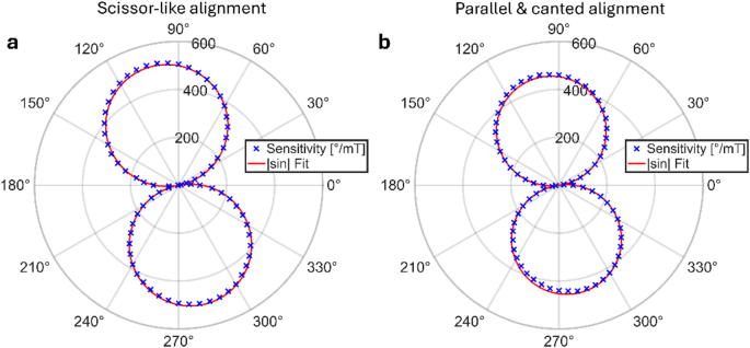
Directionality of the sensitivity with no artificial DC magnetic bias field in a 10 µT, 10 Hz AC magnetic field. Angular reference system as introduced in Fig. 3a. Fitting the data by a |sin| function calculates an 11° angular offset for the scissor-like anisotropy a), and an 8° offset for the parallel & canted alignment b).
The resulting polar plots for both the scissor-like and the parallel-and-canted configurations (Fig. 6a, b) exhibit a twofold symmetric angular dependence in a figure-of-eight pattern, which has been also reported for SAW sensors exhibiting a single magnetic layer with uniaxial anisotropy by Hu et al. 18. Displayed in red in Fig. 6, a |sin| function is fitted to the measured data. The fit reveals an angular shift of 11° for the scissor-like configuration and 8° for the parallel-and-canted anisotropy configuration. Using the same model introduced in the first section, the maximum sensitivity of the parallel-and-canted configuration with an anisotropy tilt of 14° (as obtained from the BH-loop tracer) is expected to occur at ≈ 8°. This prediction is in good agreement with the angular shift obtained from the |sin| fit and further highlights the micromagnetic aspects in determining the directional response and sensitivity of SAW magnetic field sensors. In the scissor-like configuration B-H loop tracer measurements in Fig. 4a reveal that the magnetization directions are non-collinear in remanence. However, the sensitivity recorded with an angular step size of 5° is best fitted by a |sin| function. Small deviations between sensitivity maxima at opposing angles (ΔS ≈ 3% for the scissor and ≈ 5% for the parallelly canted sensor) may be attributed to rotation within the ambient magnetic field in the unshielded environment and the known dependence of sensitivity on a static bias field (cf. Figure 5a, c).