
The time-independent Schrödinger equation
$$\hat{H}{\Psi }^{i}={E}^{i}{\Psi }^{i}\quad {\Psi }^{i}\in {{\mathcal{H}}}^{-}\,,$$
(2)
defines the electronic states of a molecule as the eigenstates Ψi of the molecular Hamiltonian \(\hat{H}\), indexed in order of increasing energy Ei. In addition, electrons are subject to the fermionic antisymmetry constraint, that is, the solutions have to belong to the antisymmetric subspace of the Hilbert space \({\mathcal{H}}^{-}\). To make the problem computationally tractable, in quantum chemistry, one commonly works in the Born–Oppenheimer approximation, neglecting spin–orbit coupling and other relativistic effects. For molecules, this approximation is implemented by the clamped-nucleus Coulomb Hamiltonian, which in first quantization (and applying atomic units) takes the form
$${\hat{H}}=-\frac{1}{2}\mathop{\sum}\limits_{i}{\nabla }_{i}^{2}-\mathop{\sum}\limits_{iI}\frac{{Z}_{I}}{| {{\bf{R}}}_{I}-{{\bf{r}}}_{i}| }+\mathop{\sum}\limits_{i < j}\frac{1}{| {{\bf{r}}}_{i}-{{\bf{r}}}_{j}| }\,,$$
(3)
with \({\nabla }_{i}^{2}\) denoting the Laplace operator, ri denoting the position of the ith electron, and ZI and RI denoting the charge and (fixed) position of the Ith nucleus. Owing to the decoupling of electronic and nuclear degrees of freedom, the Schrödinger equation holds for every molecular configuration independently, with a mere parametric dependency on the nuclei. This defines the adiabatic Born–Oppenheimer potential energy surfaces
$${\hat{H}}{\Psi }^{i}({\bf{r}}| {\bf{R}})={E}^{i}({\bf{R}}){\Psi }^{i}({\bf{r}}| {\bf{R}}).$$
(4)
Variational optimization
To approximate the eigenstates of the Schrödinger equation (2) we apply the VMC method. VMC is a variational method that minimizes the Rayleigh quotient
$${{\boldsymbol{\theta }}}^{{\prime} }=\mathop{\,\mathrm{argmin}}\limits_{{\boldsymbol{\theta }}}\frac{\langle {\Psi }_{{\boldsymbol{\theta }}}| \hat{H}| {\Psi }_{{\boldsymbol{\theta }}}\rangle }{\langle {\Psi }_{{\boldsymbol{\theta }}}| {\Psi }_{{\boldsymbol{\theta }}}\rangle }$$
(5)
of a parametrized trial wavefunction Ψθ. The goal is to find the optimal set of parameters θ′, which can then be used to evaluate expectation values. The high-dimensional integrals in equation (5) are approximated by Monte Carlo integration with importance sampling. This stochastic integration method poses very few restrictions on the functional form of the wavefunction ansatz, enabling the inclusion of explicit electronic correlation.
Throughout the optimization, expectation values are estimated on finite batches of electron samples drawn from the probability density associated with the square of the wavefunction via Markov chain Monte Carlo. At each iteration, the model parameters are updated with a flavor of stochastic gradient descent until convergence is reached. Details on the VMC method and the peculiarities of optimizing neural network wavefunctions can be found in earlier works4,16.
There are various extensions of the VMC method to target excited states. The basic requirement of these extensions is preventing the optimization from collapsing to the ground electronic state (global energy minimum), while ensuring convergence to the excited states (local energy minima). In this work, we use a penalty-based excited-state optimization method5,21, where the loss function of each state is composed of the energy of the given state plus a term penalizing its overlap with all lower-lying states. In addition, a spin penalty can be introduced to target states of a specific spin sector6,22, leading to the loss function of
$${\mathcal{L}}[{\Psi }_{{{\boldsymbol{\theta }}}_{1}},\ldots ,{\Psi }_{{{\boldsymbol{\theta }}}_{{N}_{{\rm{s}}}}}]=\mathop{\sum}\limits_{i}^{{N}_{\rm{s}}}\left[{\langle \hat{H}\rangle }^{i}+\beta {\langle {\hat{S}}^{2}\rangle }^{i}+\mathop{\sum}\limits_{j}^{j < i}{\alpha }_{ij}| \langle {\Psi }_{{{\boldsymbol{\theta }}}_{i}}| {\bar{\Psi }}_{{{\boldsymbol{\theta }}}_{j}}\rangle {| }^{2}\right]\,.$$
(6)
where \({\hat{S}}^{2}\) is the total spin operator and \(\{{{\boldsymbol{\theta }}}_{1},\ldots ,{{\boldsymbol{\theta }}}_{{N}_{{\rm{s}}}}\}\) represent the parameters of the wavefunctions corresponding to each of the Ns different states. The bar (in \(\overline{\Psi }\)) indicates that no gradient is taken with respect to the parameters of the specified wavefunction. The factor β scales the spin penalty with respect to the energy and overlap contributions and is set to a fixed value (here 10). The pairwise overlap scaling parameters αij are determined via the same expression as used in our earlier work6
$${\alpha }_{ij}=\widetilde{\alpha }\, \max\left(| {E}_{{\bf{R}}}^{i}-{E}_{{\bf{R}}}^{j}| ,\,\mathrm{ewm}(\sqrt{\mathrm{Var}({E}_{{\bf{R}}}^{\mathrm{loc},i})}),1{0}^{-3}\right),$$
(7)
where \(\tilde{\alpha } > 1\) is the additional free parameter shared between all pairs of states (set to \(\widetilde{\alpha }=4\) in all experiments reported here), ewm(⋅) denotes the exponentially weighted mean over the training iterations, \({E}_{{\bf{R}}}^{\mathrm{loc},i}\) is the batch of local energies in the current step, and Var(⋅) denotes taking the variance. The first argument of the maximum function ensures that the constraint required for obtaining orthogonal states21 is fulfilled, while automatically scaling αij in a system-specific way. The second argument prevents the collapse of the states in the earliest stages of the training where our mean energy estimates cannot yet give good approximations of the energy differences.
Transferable optimization
Typically, VMC is applied in the context of single-point calculations, that is, the parameters of the trial wavefunction are optimized to minimize the energy expectation value of a specific molecular geometry. With the vastly increased expressivity of neural network wavefunctions, however, the concept of transferable optimization has been introduced. The idea consists of sharing a subset of the wavefunction parameters across multiple geometries23 or making the ansatz explicitly dependent on the nuclear geometry24, and minimizing the energy for multiple molecular geometries simultaneously. The transferable optimization makes use of the fact that under the Born–Oppenheimer approximation equation (4) the variational principle of quantum mechanics holds independently for every nuclear configuration of a molecule, that is
$${E}_{0}({\bf{R}})=\mathop{\min }\limits_{\Psi }\frac{{\langle \Psi | \hat{H}| \Psi \rangle }_{{\bf{R}}}}{{\langle \Psi | \Psi \rangle }_{{\bf{R}}}}\le \mathop{\min }\limits_{{\boldsymbol{\theta }}}\frac{{\langle {\Psi }_{{\boldsymbol{\theta }}}| \hat{H}| {\Psi }_{{\boldsymbol{\theta }}}\rangle }_{{\bf{R}}}}{{\langle {\Psi }_{{\boldsymbol{\theta }}}| {\Psi }_{{\boldsymbol{\theta }}}\rangle }_{{\bf{R}}}}\,,$$
(8)
where \({\langle \cdots \rangle }_{{\bf{R}}}\) denotes the electronic expectation value at the nuclear geometry R. In this work, we combine the optimization across multiple molecular geometries (equation (8)) with the penalty-based loss (equation (6)) and augment the wavefunction architecture to make it more suitable to the transferable set-up. This yields geometrically transferable wavefunctions capable of describing different electronic states of a molecule across a range of molecular geometries.
We generalize the training of the wavefunction model by iterating through a dataset of molecular geometries ℜ. This amounts to minimizing the average loss (equation (6)) over the whole dataset
$${{\boldsymbol{\theta }}}^{{\prime} }=\mathop{\,\mathrm{argmin}}\limits_{{\boldsymbol{\theta }}}\sum _{{\bf{R}}\in {\boldsymbol{\Re }}}{\mathscr{ \mathcal L }}[{\Psi }_{{{\boldsymbol{\theta }}}_{1}},\ldots ,{\Psi }_{{{\boldsymbol{\theta }}}_{{N}_{{\rm{s}}}}}]({\bf{R}})\,.$$
(9)
To sample electrons for the estimation of the expectation value of the loss function at each training iteration, we use the Metropolis algorithm and keep independent Markov chains for each geometry of the dataset in memory. To retain sufficiently large electron batches (electron batch sizes) for sufficiently accurate estimates of the expectation values, we subsample the dataset of molecules and alternate between successive batches (molecule batch size). While we find the training to be fairly insensitive to the exact choice of molecule batch size, a round-robin approach with a molecule batch size of one23 can lead to the Markov chains of other molecules going stale, especially for large datasets. Therefore, when considering larger molecule datasets, a compromise between electron batch size and molecule batch size is made (Supplementary Table 12). To account for the changes of the electron distribution due to updates of the wavefunction parameters, we use a decorrelation sampler that equilibrates the Markov chains before drawing each batch of electron samples. While the approach of keeping a stack of independent Markov chains for all molecules of the dataset convinces through its simplicity, scaling to datasets with thousands of molecular geometries, it eventually hits its limitations. In these cases, the sampling can be replaced by either updating nuclear configurations within the Markov chains and warping electrons alongside the nuclei or initializing fresh Markov chains at every new molecular geometry.
Dynamic state ordering and level crossings
The penalty-based excited-state optimization implements a ladder of states approach, where collapse to the ground state is prevented by orthogonalization of excited states with respect to lower-lying states (equation (6)). The resulting order of states is of no relevance in single-point simulation and the approach guarantees the optimization of pure states, as opposed to the mixed states resulting from a symmetric loss function that penalizes both ansatzes. However, when extending the loss to a transferable setting, the order of the states gains importance, as the energy ordering might change at conical intersections and level crossings (Fig. 1, right). Albeit not strictly necessary, a continuous representation of the wavefunction along the geometries of the dataset is favorable both for model optimization in practice and for ease of interpreting the simulation results. To address this, we propose a more flexible penalty method where the direction of orthogonalization adapts based on relative energies at each configuration. We generalize the overlap penalty term of our loss function to be dependent on the nuclear coordinates as
$$\begin{array}{c}{\mathscr{ \mathcal L }}[{\Psi }_{{{\boldsymbol{\theta }}}_{1}},\ldots ,{\Psi }_{{{\boldsymbol{\theta }}}_{{N}_{{\rm{s}}}}}]({\bf{R}})=\,\ldots +\mathop{\sum}\limits_{j}^{{E}_{{\bf{R}}}^{j} < {E}_{{\bf{R}}}^{i}}{\alpha }_{ij}| {\langle {\Psi }_{{{\boldsymbol{\theta }}}_{i}}| {\overline{\Psi }}_{{{\boldsymbol{\theta }}}_{j}}\rangle }_{{\bf{R}}}{| }^{2}\\ \mathrm{where}\,{E}_{{\bf{R}}}^{j} < {E}_{{\bf{R}}}^{i}\quad {\Rightarrow }_{\mathrm{approx}.}\quad {\langle {\Psi }_{{{\boldsymbol{\theta }}}_{j}}| \hat{H}| {\Psi }_{{{\boldsymbol{\theta }}}_{j}}\rangle }_{{\bf{R}}} < {\langle {\Psi }_{{{\boldsymbol{\theta }}}_{i}}| \hat{H}| {\Psi }_{{{\boldsymbol{\theta }}}_{i}}\rangle }_{{\bf{R}}}\,,\end{array}$$
(10)
where for simplicity we omit the sums on the configurations R and on the number of states i, as they are implied. Note that the re-indexing is applied independently for every molecular configuration R ∈ ℜ. In practice, we estimate the energy expectation values of equation (10) by maintaining exponential moving averages of the training energies of each state at every geometry of the dataset. If, however, the ordering of nearly degenerate states changes during the training, the automatic scaling of αij ensures that no large, discontinuous changes are made to the loss function. By grouping states based on their physical character, this allows the network to optimize the wavefunctions more effectively.
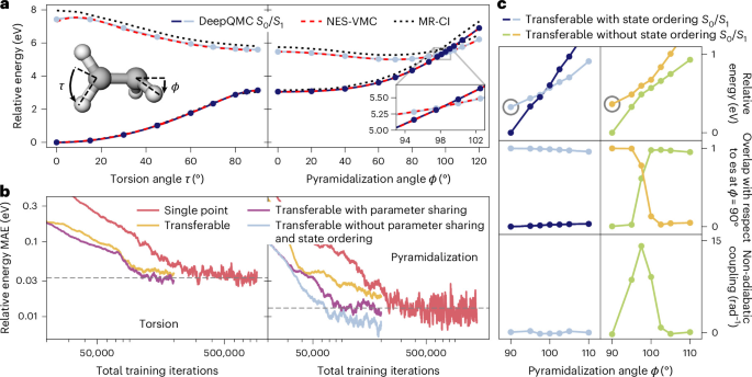
While this loss does not strictly enforce the correct ordering, we find that the continuity of the wavefunction is typically favored due to the smoothness of the neural network ansatz and enhanced optimization dynamics, as demonstrated in Fig. 1. The continuity of the wavefunctions at level crossings can be probed by evaluating intermolecular overlaps
$${O}_{{{\bf{R}}}_{m},{{\bf{R}}}_{n}}^{i,\;j}=\langle {\Psi }_{{\theta }_{i}}({\bf{r}},{{\bf{R}}}_{m})| {\Psi }_{{\theta }_{j}}({\bf{r}},{{\bf{R}}}_{n})\rangle \,,$$
(11)
between the transferable wavefunction of state i and j at nuclear configurations m and n. Figure 1c illustrates how dynamic state ordering allows the transferable network to maintain a consistent character throughout the crossing. The overlap of the excited-state wavefunction at ϕ = 90° with itself at varying ϕ remains close to 1, while its overlap with the ground state stays near 0. In contrast, without dynamic ordering, the network switches character at the crossing, causing the excited-state overlap to drop to 0 at ϕ = 100° while the overlap with the ground state rises to 1. This effect also shows in the non-adiabatic couplings between the ground state and the excited state.
Transferable wavefunction ansatz
All reported experiments were carried out using an ansatz derived from the Psiformer architecture11 that was extended to explicitly account for changes in the molecular geometry. The wavefunction \(\Psi :{{{{\mathbb{R}}}}}^{3N}\to {{{\mathbb{R}}}}\) is parameterized via the usual many-body Slater–Jastrow form
$$\Psi ({\bf{r}}| {\bf{R}})=\exp (J({\bf{r}}))\mathop{\sum}\limits_{k=1}^{{N}_{\det }}\det {\left[{\varphi }_{j}^{k}({{\boldsymbol{h}}}_{i}^{\mathrm{elec}}({\bf{r}}| {\bf{R}}))\,{\varphi}_{j}^{k}({{\bf{r}}}_{i}| {\bf{R}})\right]}^{{N}_{\mathrm{elec}}}_{i,\;j=1},$$
(12)
where \({\bf{r}}\in {{\mathbb{R}}}^{3{N}_{{\rm{elec}}}}\) are the positions of the Nelec electrons, \({\bf{r}}\in {{{{\mathbb{R}}}}}^{3{N}_{\mathrm{elec}}}\) stands for the coordinates of the Nnuc nuclei, J is a permutation-invariant Jastrow factor, \({\phi }_{j}^{k}\) are ‘generalized‘ orbitals predicted from the many-body embedding of the ith electron \({{\bf{h}}}_{i}^{{\rm{elec}}}\), and \({\varphi }_{j}^{k}({{\mathbb{r}}}_{i}| {\bf{R}})\) are single-electron envelope functions anchored at the nuclei. The determinant of the Nelec × Nelec orbital matrix enforces fermionic antisymmetry, and the Ndet such determinants are summed to increase the expressivity of the ansatz. Following the standard convention in variational Monte Carlo calculations for molecular systems, we use spin-assigned wavefunctions in which the first N↑ electrons are assigned spin up and the remaining \({N}_{\mathrm{elec}}^{{\rm\downarrow }}={N}_{\mathrm{elec}}-{N}_{\mathrm{elec}}^{{\rm\uparrow }}\) electrons are assigned spin down. Consequently, the fixed spin configuration does not appear as an explicit argument of the wavefunctions but is incorporated implicitly through the spin assignment.
At the core of the wavefunction is the self-attention neural network architecture, which encodes the electron configuration in a latent space. To that end, initial per-electron and per-nucleus feature vectors are constructed from rescaled electron–nuclei and nuclei–nuclei distances, electron spins and nuclei charges, respectively
$${{\bf{h}}}_{i}^{\mathrm{elec},0}={\mathrm{MLP}}_{\mathrm{embed}}^{\mathrm{elec}}\left(\mathop{\oplus}\limits_{I=1}^{{N}_{\mathrm{nuc}}}(s({{\bf{r}}}_{i}-{{\bf{R}}}_{I}),\,s(| {{\bf{r}}}_{i}-{{\bf{R}}}_{I}| )),{\sigma }_{i},\right)$$
(13)
$${{\boldsymbol{h}}}_{I}^{{\rm{nuc}},0}={{\rm{MLP}}}_{{\rm{embed}}}^{{\rm{nuc}}}\left(\sum _{{I}^{{\prime} }}{{\rm{MLP}}}^{{\rm{edge}}}\left(\left(s({{\bf{R}}}_{I}-{{\bf{R}}}_{{I}^{{\prime} }})\oplus \,s(| {{\bf{R}}}_{I}-{{\bf{R}}}_{{I}^{{\prime} }}| )\oplus {Z}_{I}\right)\right)\right)\,,$$
(14)
where ⊕ is the concatenation operation, σi ∈ {+1, −1} is the electron spin, \({Z}_{I}\in {\mathbb{Z}}\) are the nuclear charges and MLP denotes multi-layer perceptrons. The function s(⋅) corresponds to a logarithmic rescaling of the distances and differences
$$s({\bf{R}})=\frac{\mathrm{log}(1+| {\bf{R}}| )}{| {\bf{R}}| }{\bf{R}}\,,$$
(15)
increasing the numerical stability of the model at large interparticle distances. Each layer then updates the embeddings via multi-headed (causal) self-attention with residual connections
$${{\bf{f}}}_{i}^{\ell +1}={{\bf{h}}}_{i}^{\ell }+{W}_{o}^{\ell },\mathop{\bigoplus}\limits_{h}\left[\frac{1}{\sqrt{d}}\mathop{\sum}\limits_{j}{\mathrm{softmax}}_{j}({({{\bf{q}}}_{i}^{\ell h})}^{T}{{\bf{k}}}_{1}^{\ell h},\ldots ,{({{\bf{q}}}_{i}^{\ell h})}^{T}{{\bf{k}}}_{{N}_{\mathrm{elec}}}^{\ell h}){{\bf{v}}}_{j}^{\ell h}\right]$$
(16)
$${{\bf{h}}}_{i}^{\ell +1}={{\bf{f}}}_{i}^{\ell +1}+\tanh \left({W}^{\ell +1}{{\bf{f}}}_{i}^{\ell +1}+{b}^{\ell +1}\right)\,,$$
(17)
with keys, values and queries given by
$${{\bf{q}}}_{j}^{\ell h}={W}_{q}^{\ell h}{{\bf{h}}}_{j}^{\ell },\qquad {{\bf{k}}}_{j}^{\ell h}={W}_{k}^{\ell h}{{\bf{h}}}_{j}^{\ell },\qquad {{\bf{v}}}_{j}^{\ell h}={W}_{v}^{\ell h}{{\bf{h}}}_{j}^{\ell }$$
(18)
and softmaxj(⋅) being the softmax function
$${\mathrm{softmax}}_{j}({x}_{1},\ldots ,{x}_{n})=\frac{\exp ({x}_{j})}{{\sum }_{i}\exp ({x}_{i})}\,.$$
(19)
The weight matrices \({W}_{(\cdot )}^{\ell }\) and bias vectors bℓ hold the trainable parameters of the ℓth layer of the encoder and d is the dimension of the key, query and value vectors. In multi-headed self-attention several independent heads, indexed by h, are evaluated and concatenated. Inspired by the Born–Oppenheimer approximation, we improve the efficiency of the Laplacian computation for the electronic degrees of freedom by restricting nuclear message passing to nuclear–nuclear interactions, while allowing nuclei to provide their states to electrons. After several layers of interactions the final many-body embeddings of the electrons are projected to obtain the generalized orbitals \({\phi }_{j}^{k}={W}_{\mathrm{orb}}{{\bf{h}}}_{i}^{\mathrm{elec}}\). At the same time, from the final nucleus representations the envelope exponent parameters ζIjkn are predicted, by passing them through a gated linear unit with sigmoid activation.
To remedy the memory bottleneck induced by the computation of the orbital envelope functions \({\varphi }_{j}^{k}\) (refs. 7,9), we use envelopes similar to the simplified envelopes in ref. 9, that is, we compute the envelopes as
$${\varphi }_{j}^{k}({{\bf{r}}}_{i})=\sum _{I}^{{N}_{\mathrm{nuc}}}\sum _{n}^{3}\exp (-{\zeta }_{Ijkn}| {{\bf{r}}}_{i}-{{\bf{R}}}_{I}| )\,,$$
(20)
where I sums over nuclei and n indexes a total of three envelopes per nucleus.
Furthermore, because self-attention does not directly access pairwise electron distances, it is not well suited to capture the electron–electron cusp condition. We therefore augment it with a simple two-parameter Jastrow factor that enforces the cusp condition analytically
$$J({\bf{r}})=\mathop{\sum}\limits_{i < j;\,{\sigma }_{i}={\sigma }_{j}}-\frac{1}{4}\frac{{\alpha }_{\mathrm{par}}^{2}}{{\alpha }_{\mathrm{par}}+| {{\bf{r}}}_{i}-{{\bf{r}}}_{j}| }\,+\,\mathop{\sum}\limits_{i,\;j;\,{\sigma }_{i}\ne {\sigma }_{j}}-\frac{1}{2}\frac{{\alpha }_{\mathrm{anti}}^{2}}{{\alpha }_{\mathrm{anti}}+| {{\bf{r}}}_{i}-{{\bf{r}}}_{j}| }\,.$$
(21)
The cusp parameters are trainable and initialized with \({\alpha }_{\mathrm{par}}=\frac{1}{4}\) and \({\alpha }_{\mathrm{anti}}=\frac{1}{2}\).
Parameter sharing between electronic states
Parameter sharing has been demonstrated to be very efficient when transferably simulating ground states by exploiting similarities in the wavefunctions of different molecular configurations. Analogous similarities may arise when simulating multiple electronic states of a molecule, for instance, due to the presence of core orbitals, which are not involved in any of the electronic excitations. While previous studies used distinct sets of model parameters for each excited state respectively5,6, we propose to share a large fraction of the model parameters between the states
$${\Psi }_{{{\boldsymbol{\theta }}}_{1}}({\bf{R}}),\ldots ,{\Psi }_{{{\boldsymbol{\theta }}}_{{N}_{{\rm{s}}}}}({\bf{R}})\to {\Psi }_{({{\boldsymbol{\theta }}}_{1},{{\boldsymbol{\theta }}}^{{\rm{s}}})}({\bf{R}}),\ldots ,{\Psi }_{({{\boldsymbol{\theta }}}_{{N}_{{\rm{s}}}},{{\boldsymbol{\theta }}}^{{\rm{s}}})}({\bf{R}})\,.$$
(22)
The parameter sharing is implemented by averaging a subset of the model parameters after each gradient update. Supposing that there is appreciable similarity between the wavefunctions of different states, parameter sharing improves error cancellation on relative energies by correlating the latent space representation of electrons in the wavefunctions of different states and effectively increases the number of gradient steps the shared parameters receive. It is important to note that parameter sharing across electronic states is considered a useful tool for reducing simulation costs. However, it is neither necessary to attain high accuracy nor guaranteed to improve convergence, in a manner similar to related concepts such as state averaging in CASSCF or frozen-core orbitals in equation-of-motion coupled-cluster (EOM-CC). Furthermore, the optimal parameter-sharing strategies may depend on the electronic structure of the system under investigation and could, in principle, vary across the simulated geometries. We empirically determine that such dependence is negligible. On the basis of our experiences, we recommend sharing the entire self-attention mechanism. Occasionally, sharing large fractions of the parameters and thereby reducing the per-state expressivity of the ansatzes can hinder convergence to the correct set of states. To account for these outliers, parameter sharing can be turned off at any time throughout the optimization or the effect can be remedied by reducing the fraction of shared model parameters, for instance, sharing only the initial layers of the self-attention block.
As parameter sharing and pseudopotentials leverage related similarities between electronic states, the benefits of sharing parameters may be reduced when comparing simulations with pseudopotentials to their (generally more expensive) all-electron counterpart. At the same time, we did not observe a deterioration of the accuracy in relative energies when combining parameter sharing with pseudopotentials. An extended analysis of the parameter sharing across electronic states for the ethylene pyramidalization can be found in Supplementary Information, section 4.
Pseudopotentials and pseudohamiltonians
While core electrons contribute dominantly to the total energy, they are chemically inert, with most chemical and bonding properties governed by valence electrons. By removing the core electrons and representing their effect through pseudopotentials, the number of active electrons is reduced, leading to faster convergence and improved stability. This simplification also smoothens the valence wavefunction, enhancing the efficiency of Monte Carlo sampling by allowing larger step sizes, and the reduced electron count reduces the memory requirements and speeds up convergence of the wavefunction.
A typical pseudopotential, such as ccECP15 ued for the methylenimmonium cation calculations, replaces the nuclear Coulomb potential (second term in equation (3)) with a non-local operator acting on the angular momentum components of the wavefunction (see ref. 16 for details). Although this substitution greatly simplifies the physical problem, it introduces computational overhead due to the additional integrals introduced by the non-local operators, which we approximate using a 12-point quadrature scheme. Recently, local forms of pseudopotentials have been introduced in the context of deep-learning QMC19, and are used here to model the rubredoxin active site. Such local pseudopotentials, also termed pseudohamiltonians, circumvent the costly non-local integrals while maintaining a comparable level of accuracy. This represents a further substantial improvement in computational efficiency, thereby enabling the scaling of DeepQMC calculations to systems of considerable size.
Accuracy metric
Throughout, accuracy is quantified by the MAE of relative energies. As total energies are less chemically relevant and not as directly comparable across methods, we assess relative energies, that is, energy differences across geometries and electronic states. For a set of geometries {R} and states i, the MAE is computed between the DeepQMC energies \({E}_{{\bf{R}}}^{i}\) and the reference energies \({\tilde{E}}_{\bf{R}}^{i}\) after aligning the two sets by a single constant shift, chosen such that their mean energies across all included geometries and states coincide
$$\mathrm{MAE}=\frac{1}{N}\sum _{{\bf{R}},i}| {E}_{{\bf{R}}}^{i}-{\tilde{E}}_{\bf{R}}^{\;i}-\Delta | ,\qquad \Delta =\frac{1}{N}\mathop{\sum}\limits_{{\bf{R}},i}({E}_{{\bf{R}}}^{i}-{\tilde{E}}_{\bf{R}}^{\;i}),$$
(23)
where N is the number of geometry-state pairs included in the average. This single global shift removes the arbitrary constant offset between methods while preserving all relative energies.
Non-adiabatic couplings
The continuity of the transferable wavefunctions across level crossings can be characterized through the intermolecular overlaps of equation (11) and the resulting non-adiabatic couplings (NACs), which are central to surface-hopping simulations. The NAC between states i and j along a nuclear coordinate—on the ethylene simulation (Fig. 1), we chose the pyramidalization angle ϕ—is the overlap gradient
$${h}_{ij}(\phi )={\nabla }_{{\phi }^{{\prime} }}\langle {\Psi }_{i}(\phi )| {\Psi }_{j}({\phi }^{{\prime} })\rangle {\left\vert \right.}_{\phi = {\phi }^{{\prime} }},$$
(24)
which we approximate by finite differences20
$${h}_{ij}(\phi )\approx \frac{1}{2{\Delta }\phi }(\langle {\Psi }_{i}(\phi )| {\Psi }_{j}(\phi +{\Delta }\phi )\rangle -\langle {\Psi }_{i}(\phi )| {\Psi }_{j}(\phi -{\Delta }\phi )\rangle ),$$
(25)
using a non-uniform step Δϕ set by the spacing of the geometry dataset. Here we evaluate the coupling along the nuclear coordinate, with the time-derivative coupling that would enter the surface-hopping equations in molecular dynamics followed by contraction with the nuclear velocity, \(\langle {\Psi }_{i}| {\partial }_{t}{\Psi }_{j}\rangle =\langle {\Psi }_{i}| {\nabla }_{{\bf{R}}}{\Psi }_{j}\rangle \cdot {\dot{\bf{R}}}\). With dynamic state ordering, the transferable simulations yield quasi-diabatic representations, that is, electronic states that remain continuous along the one-dimensional cut through the conical intersection. Their overlaps stay close to one within a state and close to zero between states across the crossing, so the NACs remain small. With a fixed ordering, by contrast, the states flip character at the crossing, producing a discontinuity in the overlaps and pronounced spurious couplings.
Computational set-up
All presented simulations are run with the DEEPQMC software package16,25, which provides JAX implementations of the core algorithms with graphics processing unit acceleration and multi-node parallelization. Parameter updates are computed using the KFAC algorithm26. For the efficient computation of the kinetic energy operator \({\sum }_{i}{\nabla }_{i}^{2}\) we use automatic differentiation and use the forward Laplacian framework27. All experiments were run on NVIDIA-A100 graphics cards on the supercomputer Lise at NHR@ZIB.
Reporting summary
Further information on research design is available in the Nature Portfolio Reporting Summary linked to this article.