
Few-shot learning-driven slope streak mapping
I build on the validated slope streak detector (based on YOLOv5, PyTorch 1.7, from https://github.com/ultralytics/yolov5) used in ref. 7 and substantially improve its overall detection performance by adding a total of 4737 and 389 new slope streak labels located in a total of 575 and 41 CTX image patches (1000 × 1000 pixels each), for training and testing data, respectively, taken from 27 CTX images. The full, used training and testing datasets include 5744 and 424 streak labels taken from 68 CTX images. Each label represents one rectangular bounding box drawn around a slope streak. Data selection, labeling, and validation, as well as detector training, follow the identical procedures as documented by Bickel and Valantinas7, including label augmentation (label rotation, up-down flipping, shearing, scaling, and contrast/brightness modifications), which in turn followed established procedures. All used CTX images are listed in Table S1.
The trained detector achieves a recall of ~75% (% streaks in testset identified) and a precision of ~94% (% correctly identified testset streaks) at a model confidence threshold of 0.5, with an AP (average precision) of ~80%. The detectors used by Bickel and Valantinas7 and in this work cannot be directly compared due to their different testsets, but the performance of the new detector is expected to be substantially enhanced, due to the considerably larger and more diverse trainset. The test results imply that the detector is able to identify about 75% of all streaks visible in a CTX image, while about 94% of its detections are correct, on average. For this study, I deploy the new detector with a confidence threshold of 0.5, i.e., I consider all detections with model confidence scores higher than 0.5. Due to the fact that individual streaks can be spatially co-located or overlap (nested streaks), I use a random set of 1000 streaks to estimate the average number of slope streaks per detection: ~2 (slightly lower than the ~2.33 estimated by Bickel and Valantinas7, most likely due to the improved detector).
The deployment of the detector uses the identical methodology as detailed in ref. 7, utilizing one single NVIDIA RTX 3090 GPU (Graphical Processing Unit) and a processing pipeline developed over several years (e.g., refs. 48,49). The workflow retrieves map-projected and calibrated CTX images located between 55°N and 35°S (n = 105,754, geographically constrained by the earlier global census conducted by Bickel and Valantinas7) from https://image.mars.asu.edu/stream/, cuts them into 1000 × 1000 pixel patches, deploys the detector, and uses the standard YOLOv5 NMS (non-maximum suppression) to remove duplicate detections made in the same image patch, as is best practice for object detection. All detections are stored along with preview thumbnails and CTX-derived metadata, such as accurate geographic location, image solar longitude, image ID, image acquisition date, illumination conditions, and imaging geometry. Total processing of the entire (available) CTX image archive required ~1.5 months using one single GPU-enabled desktop computer. The detector identified a total of 2,169,234 individual slope streak detections, which are too many for a manual candidate review, as performed by Bickel and Valantinas7; in this study, I rely on the thorough (statistical) assessment of the precision of the detector in the testset: this assessment suggests a precision of 94%, which means that a minimal number of false detections are included in the dataset, but strongly implies that those false detections will not have any substantial effect on the scientific results and interpretations. A purely statistical assessment of detector precision – without manual review – is common for datasets with extremely large numbers of detections, such as recently showcased in ref. 50, which mapped millions of boulders across the lunar surface.
Spatiotemporal data binning and statistics
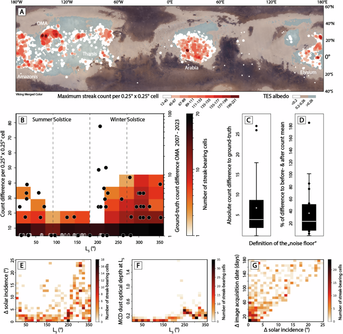
I use a geographic grid consisting of 520,200 0.25° × 0.25° quadrangles that cover Mars between 55°N and 35°S. Each slope streak detection is associated with the unique ID of its ‘host cell’ or ‘analysis cell’. The spatiotemporal analysis is conducted on a cell-by-cell basis. Overall, I consider 91,687 CTX images. On average, each analysis cell intersects with 6.52 CTX images, with a minimum of 1 image and a maximum of 187 images. The used CTX images feature a homogeneous longitudinal distribution and a relatively homogeneous latitudinal distribution, with fewer images taken at very high northern latitudes, beyond ~45°N (Fig. S3). Past surveys have not identified any slope streaks at latitudes beyond ~40°N (e.g., ref. 7). The used CTX images feature a slightly heterogeneous seasonal distribution, with more images acquired over northern spring and summer (LS~0° to ~170°) and fewer images over southern spring, summer, and autumn (LS~220° to ~360°) (Fig. S3). The relative lack of images is particularly expressed at very high northern latitudes, beyond ~40°N, between ~200° and ~360° LS, where no slope streaks are present. It is unlikely that the seasonal imbalance of images has an effect on the results of this study, as the overabundance of images in northern spring and summer should affect the streak counts at those seasons, yet the peak streak formation season is associated with southern spring, summer, and autumn (Fig. 1B).
Maximum counts
This workflow uses the slope streak counts made by the detector in a given cell, in all CTX images that fully or partially overlap that cell. The workflow selects the overall maximum count made in each cell; in other words, the workflow derives the largest number of slope streaks ever recorded by CTX in a given cell. In addition, the workflow extracts the maximum (annual) climatology average solar MY horizontal wind velocity (\({U}_{x}\)) at an altitude of 4.5 m above the surface (z), a daily column-integrated dust optical depth value (regularly kriged maps of 9.3 μm absorption column dust optical depth, 610 Pa51), as well as the atmospheric density (\({\rho }_{a}\)) at the respective time from the MCD25,52. I use those parameters along with the law of the wall33 to compute the wind shear velocity (\({u}_{*}\)) at surface level (with κ as the von Kármán constant, 0.4, and \({z}_{0}\) as the aerodynamic surface roughness, here 2 cm):
$$\overline{{U}_{x}}\left(z\right)=\frac{{u}_{ * }}{\kappa }\mathrm{ln}\left(\frac{z}{{z}_{0}}\right)$$
(1)
and then estimate the wind stress (\(\tau\)) using28,33:
$$\tau={\rho }_{a} * {u}_{ * }^{2}$$
(2)
\({z}_{0}\) is computed using (per, e.g., ref. 39):
$${z}_{0}=2 * \frac{D}{30}$$
(3)
assuming a median grain size (D) of 30 cm, as recently used by Bickel et al. 34. I note that the utilization of one single D and \({z}_{0}\) value as well as the usage of Eq. (3) largely oversimplifies the substantial variability of the aerodynamic roughness across Mars. Most notably, the assumed D and \({z}_{0}\) values are relatively high and might not be fully representative for many slope streak-bearing regions.
Wind stress values beyond ~0.02 Pa, either vortical (e.g., in dust devils or convective vortices)53,54,55 or non-vortical (e.g., in near-surface wind gusts)28,34 have been shown to be able to initiate and sustain the saltation of sand-sized particles (~100 µm), which can eject finer dust-sized particles upon re-impact on the surface. The ejection of dust through saltating sand-sized particles is suspected to be the main dust lifting mechanism on Mars (e.g., ref. 33,56,57,58,59,60). Lastly, the workflow extracts the TES albedo61 and MOLA topographic elevation62,63 at each streak location.
Differential counts – seasonal
This workflow selects all CTX images that have a 100% overlap with a given cell, i.e., the process excludes images that might only partially cover a given cell, which likely leads to lower counts. Subsequently, the workflow identifies image pairs with a temporal acquisition difference of less than 6 months (one quarter MY, 90° LS), counts slope streaks in the before and after image, and computes a count difference, embodying an integration of the number of streaks that formed and faded between the two images. I identify 6 months as the most appropriate time difference (time window) for this analysis, as it represents the best compromise between data availability and temporal resolution, i.e., identified changes can be attributed to a season with reasonable accuracy – yet, the temporal window is wide enough to maximize the number of image pairs available, which in turn improves the overall spatiotemporal coverage of the analysis.
The slope streak counts can be substantially affected by the illumination and observation geometries of the available images, as well as their overall data quality and the state of the Martian atmosphere (e.g., atmospheric dust, Fig. 1C, D, S1). In fact, the conditions that mainly drive detections of false changes (solar incidence and atmospheric dust) are more prevalent during the southern summer and fall, which might affect the results of the presented change detection analysis. I carefully characterize the noise floor caused by false changes in a statistical manner by comparing detector- and human-derived (ground-truth) streak counts in 100 control cells across the five streak hotspots. The median absolute difference between detector- and human-derived change counts (i.e., counts of newly formed streaks) is 4 per cell per pair (Fig. 1C). As the total number of streaks per cell can vary drastically and as streaks can be nested, I define the noise floor as the median percentage of the difference between the human-derived count difference and the detector-derived count difference and the mean of the detector-derived before and after image counts, i.e., ~24% (Fig. 1D). This study only considers difference counts that exceed the median noise floor, to minimize the impact of false changes, acknowledging that the application of the noise floor reduces the overall sensitivity of the investigation to subtle, small-scale changes. Importantly, even changes beyond the noise floor can be caused by data quality issues or differences (Fig. 1C, D), which remains the most relevant limitation of the overall accuracy of the presented results. Notably, tightening the requirements on, for example, incidence and temporal differences between CTX images drastically reduces the overall number of cells with appropriate spatiotemporal coverage, impeding a representative, global-scale change detection analysis (Fig. 1G). My analysis does not consider the fading of slope streaks (negative formation rates), as the signature of fading streaks is less clearly defined (i.e., is not binary, as in the streak formation case, e.g., ref. 12) and is thus substantially less pronounced in the count data, and is also noticeably more affected by count noise.
For all cells with slope streaks, the workflow further uses the average LS of a given image pair to extract a daily column-integrated dust optical depth value (regularly kriged maps of 9.3 μm absorption column dust optical depth, 610 Pa) from the MCD51. The workflow also extracts the maximum (regional, averaged) horizontal wind velocity value (at an altitude of 4.5 m above the surface) that is predicted by the MCD for the given sol, at the given LS and the given MY, as well as the corresponding atmospheric density value25,52. As for the maximum count workflow, I use those parameters to compute the wind shear velocity at the surface level and to estimate the resulting wind stress. As a last step, the workflow extracts the TES albedo61 and MOLA topographic elevation62 at all streak locations.
Differential counts – non-seasonal
This workflow focuses on all cells that contain (a) slope streaks and (b) a new impact that formed during CTX operations (n = 1027, based on ref. 23) or an InSight epicenter location (n = 24, BB ‘Broadband’ and LF ‘Low-Frequency’ events with back-azimuth, InSight MQS Catalog v14)20,21. InSight BB and LF events are classified as tectonic events41,64. If a cell contains a quake epicenter, all adjacent 8 cells are also included in the analysis, to broaden the spatial footprint of the overall analysis. The workflow considers all CTX images that overlap a given cell at least by 90%, counts slope streaks in each image, and plots all counts as a function of time (Fig. 2E), along with the temporal brackets derived by Daubar et al. 23 for each impact event – or along with the exact timing of a given quake, as provided by the MQS Catalog v1420. The utilization of a 90% overlap criterion slightly increases the count noise but substantially increases the number of images available for the analysis. I manually analyze each of the cell time-series, looking for subtle to stark increases in the streak counts that could be related to an impact or seismic event.
Manual ground-truth counts
In order to validate all automated maximum and difference counts, I conduct a detailed manual slope streak time-series analysis of two separate cells centered at 24°N, 147°W and 28°N, 145°W, in OMA. The analysis uses a total of 40 and 26 CTX image pairs, respectively, that feature 100% overlap with the cell and feature temporal differences of less than 6 months, acquired as part of a monitoring campaign between 2007 and 2023. This workflow resembles the differential count workflow, (manually) counts slope streaks in before and after images, per image pair, computes count differences, and records them along with the average LS of the respective CTX image pair (Fig. 1B).
Formation rates
I use an adapted workflow to derive slope streak formation rates on MY-scales. This workflow utilizes all CTX images that have a 100% overlap with a given cell, selects the two images with the largest temporal difference (with a maximum difference of ~17 years or ~8.5 MY, ~2007 to ~2024), counts slope streaks in the before and after image, and computes the count difference. The workflow uses two approaches to compute slope streak formation rates: (1) one approach relates the number of streaks that formed between the before and after image to their temporal difference, providing a measure of ‘newly formed slope streaks per MY’ (\({N}_{c}\)):
$${N}_{c}=\frac{{N}_{{dif}{f}_{{count}}}}{{\Delta }_{t}}$$
(4)
Notably, the number of newly formed streaks is dependent on the overall abundance of slope streaks in a given cell (see, e.g., ref. 15), which is why approach (2) relates each difference count to the total number of slope streaks that are present in the after image (\({N}_{{total}}\)), providing a measure of ‘percentage of population-increase per MY’ (\({N}_{n}\)), directly following the methodology developed and used by12,16,17,18:
$${N}_{n}=\frac{{N}_{{diff}{\rm{\_}}{count}}}{{\Delta }_{t} * {N}_{{total}}} * 100$$
(5)
Methodological and data limitations
The most important limitation of the accuracy of the presented results is the noise caused by (a) the slope streak counts and (b) the temporal bias introduced by the applied CTX image pair window (6 months), which in turn are rooted in the variability of the available CTX image data, as discussed above. In addition, there are other factors that affect the accuracy of the results presented throughout this work. The spatiotemporal analysis relies on various auxiliary datasets and model-derived products, specifically, TES surface albedo61, MOLA topographic elevation62,63, catalogs of new impact craters23 and marsquakes20,21, and the MCD25,52. Each of those products is subject to different limitations that might affect the results of this study. For example, the used catalogs of new impacts and marsquakes are very likely incomplete, in space and time, as demonstrated by recent studies that identified additional impact events (see, e.g., ref. 65). InSight data, in particular, is extremely scarce in space and time, and only features minimal overlap with the other datasets used. TES and MOLA products feature spatial resolutions that are not representative of the local, meter-scale environment that is likely to play an important role in slope streak pre-conditioning and triggering. The MCD only provides approximate, low-resolution, region-scale (5.625° longitude by 3.75° latitude per cell), and thus heavily averaged insights into atmospheric processes, and cannot be expected to fully represent the dynamic, complex topographic environments slope streaks are located in. Recent work showed that the MCD appears to substantially underestimate the horizontal near-surface wind velocity34, which implies that this work underestimates the wind stresses at slope streak locations. I underline the importance of local and regional studies – and the utilization of high-resolution products and meso-scale atmospheric models, in combination with the new dataset that is associated with this study – for the future verification and scrutiny of the results presented here, as previously highlighted by Bickel and Valantinas7.