
Yield calculations and their experimental validation
As discussed in the main text, we consider design parameters consisting of the chemical potentials μα of each particle species α and the binding energies εαβ,ij between sites i and j of particle species α and β, where a positive εαβ,ij indicates an attractive interaction. To simplify the notation, we collect the chemical potentials and non-zero binding energies in a parameter vector:
$${\bf{\xi }}=\frac{1}{{k}_{{\rm{B}}}T}\left[\begin{array}{c}{\mu }_{1}\\ \vdots \\ {\mu }_{{n}_{{\rm{spc}}}}\\ {\varepsilon }_{{\alpha }_{1}{\beta }_{1},{i}_{1}\;{j}_{1}}\\ \vdots \\ {\varepsilon }_{{\alpha }_{{n}_{{\rm{bnd}}}}{\beta }_{{n}_{{\rm{bnd}}}},{i}_{{n}_{{\rm{bnd}}}}{j}_{{n}_{{\rm{bnd}}}}}\end{array}\right]$$
(7)
where nspc is the number of particle species and the nbnd allowed bonds are defined by the binding rules (for example, Fig. 1b). ξ has dimension d = nspc + nbnd. The vector Ms that appears in equation (1) counts the number of species and bond types present in structure s. If the structure contains \({n}_{s}^{\alpha }\) particles of species α, and \({b}_{s}^{\alpha \beta ,ij}\) bonds connecting binding sites i and j of species α and β, then
$${{\bf{M}}}_{s}=\left[\begin{array}{c}{n}_{s}^{1}\\ \vdots \\ {n}_{s}^{{n}_{{\rm{spc}}}}\\ {b}_{s}^{{\alpha }_{1}{\beta }_{1},{i}_{1}{j}_{1}}\\ \vdots \\ {b}_{s}^{{\alpha }_{{n}_{{\rm{bnd}}}}{\beta }_{{n}_{{\rm{bnd}}}},{i}_{{n}_{{\rm{bnd}}}}{j}_{{n}_{{\rm{bnd}}}}}\end{array}\right]$$
(8)
The pre-factor Ωs is the entropic partition function of a structure s, and is given by
$${\varOmega }_{s}=\frac{{Z}_{s}^{{\;\rm{vib}}}\,{Z}_{s}^{{\;\rm{rot}}}}{{\lambda }^{{D}{n}_{s}}{\sigma }_{s}},$$
(9)
where \({Z}_{s}^{{\rm{vib}}}\) and \({Z}_{s}^{{\rm{rot}}}\) are the vibrational and rotational partition functions33,34 of s, respectively; λD is the volume of a phase-space cell; and \({n}_{s}={\sum }_{\alpha }{n}_{s}^{\alpha }\) is the number of particles in s. The symmetry number σs counts the number of permutations of particles in s that are equivalent to a rotation of the structure33. The multiplicity coming from the permutations of identical particle species is taken into account implicitly through the chemical potentials27,34,41. If the microscopic interactions between particles are known, Ωs can be computed using the methods in refs. 33,34,35,44.
We assume Ωs to be independent of ξ, which is exactly true for simple interaction models, such as those in ref. 27, and a good assumption in general, since the effect of the parameters on structure entropy is much weaker than their contribution in the Boltzmann weight (equation (1)). For the DNA-origami particles that we study here, models of the DNA-mediated binding interactions suggest that the binding entropy and energy can, to some extent, be tuned independently17.
When enumerating the structures in this paper, we assume that bond stiffness is very high, such that building blocks can only fit together side by side and strained structures cannot form. This assumption could be relaxed27, in which case the partition function for a strained structure would carry an additional factor \({\rm{e}}^{-{\varepsilon }_{{\rm{strain}}}/kT}\), set by the strain energy εstrain. As long as this strain energy does not strongly depend on, or is linear in, the design parameters, our framework applies to strained structures as well.
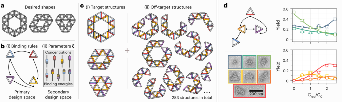
Figure 1d shows that equilibrium yields, as predicted by equation (2), agree excellently with the experimental yields. We have realized the particles and binding rules shown in Fig. 1d (left) with DNA origami (the details of which are discussed below and in Supplementary Information, section 2), and we measured the yields of the seven possible structure shapes as a function of the concentration cred of the particle species shown in red. All other particle species were kept at cblue = cyellow = cpurple = c0, with c0 = 2 nM. We measure the yields by counting the occurrence of each structure shape in the TEM images (excluding occasional unidentifiable aggregates), as shown in Supplementary Fig. 6 and Supplementary Table 3. At each value of cred, we obtain between 300 and 700 structure counts, leading to n = 3,617 structure counts in total. The binding energies of all the four bond types were designed to be the same in the experiments. Because the precise value of the binding energy is unknown, we use it as a fit parameter in our theoretical calculations. Minimizing the least-squares error between the yields predicted by equation (2) and the experimental yields, while constraining the values of the chemical potentials to reproduce the experimental particle concentrations, we obtain optimal agreement at a fitted binding energy of approximately 12.1kBT, as discussed in the main text.
For the measured yields shown in Fig. 1 and Fig. 4, we compute the error bars as follows. For a given collection of structure counts ns, the experimental (relative) yield of structure s is defined as
$${Y}_{s}=\frac{{n}_{s}}{N}$$
(10)
where N = ∑sns is the total number of structure counts. Assuming that the counting errors are given by the square roots of the counts, we estimate the error of the yields via
$$\Delta {Y}_{s}\approx \sqrt{\sum _{{s}^{{\prime} }}{\left(\frac{\partial {Y}_{s}}{\partial {n}_{{s}^{{\prime} }}}\right)}^{2}{n}_{{s}^{{\prime} }}}=\sqrt{\frac{{n}_{s}}{{N}^{2}}-\frac{{n}_{s}^{2}}{{N}^{3}}}$$
(11)
Structure enumeration
Most of the results in this paper were obtained with help from the structure enumeration algorithm introduced in ref. 27, which is capable of efficiently generating structures in two or three dimensions that satisfy a given set of binding rules, assuming rigidly locking binding interactions. The algorithm enumerates all physically realizable structures that can be formed from the given binding rules, meaning that steric overlaps and bonds between incompatible binding sites are forbidden. Particle overlaps are easily detected for particles assembling on a lattice (as is the case in all systems shown here); more complex building blocks can, in principle, be represented as rigid clusters of spheres or triangulated meshes to find overlaps and contacts27.
The algorithm can enumerate roughly 10,000 structures per second, and all enumerations in this paper were performed in less than 1 s on a 2024 MacBook Pro. The algorithm makes it possible to quickly detect whether a given set of binding rules leads to infinitely many structures or not, and can optionally generate structures only up to a maximal size. It is, in principle, possible to extend the enumeration algorithm to enumerate structures with flexible bonds. This would require a model of the microscopic binding interactions between particles, and would lead to additional computational costs27.
It is important to note that our theory is completely agnostic towards what enumeration method is used, and in general, the best (that is, most efficient or convenient) method for generating structures depends on the system at hand. For example, very different algorithms have been used to enumerate rigid sphere clusters39,44,56, or conformations of colloidal polymers40.
Thermodynamic constraints
To see why diverging structure densities in the asymptotic limit are unphysical, note that for the parameters violating \({{\bf{M}}}_{s}\cdot \hat{{\bf{\xi }}}\le 0\), particle concentrations rise as λ is increased, meaning that to realize the asymptotic limit, more and more particles need to be added to the system. At some point, steric effects between structures, which are not explicitly modelled here, make it impossible to add more particles, which means that the chemical potentials cannot be raised further, making it impossible to reach the asymptotic limit.
This situation is similar to, but distinct from, other cases in which unphysical chemical potentials emerge, such as standard aggregation theory37, or, for example, degenerate Bose gases41. In these cases, unphysical chemical potentials arise owing to singularities in the partition function, whereas in our case (assuming a finite number of possible structures), the forbidden chemical potentials come from the imposition of the asymptotic limit in parameter space.
Designability in the canonical ensemble
In the main text, we have described the assembly process using the grand canonical ensemble, which is the most convenient for our yield calculations. In practice, however, assembly usually happens in the canonical ensemble, meaning that particle concentrations, and not chemical potentials, are held constant.
In the thermodynamic limit (meaning that there are a large number of particles in the system), which is a good approximation for most self-assembly experiments, the canonical and grand canonical ensembles are equivalent41. This means that the equilibrium state described in the grand canonical ensemble by some choice of chemical potentials μα is equivalent to the state described in the canonical ensemble by specifying the total particle concentrations ϕα, provided the chemical potentials and particle concentrations are related via
$${\phi }_{\alpha }=\sum _{s\in {\mathcal{S}}}{n}_{s}^{\alpha }{\rho }_{s}({\mu }_{\beta })$$
(12)
where the sum runs over all possible structures s, \({n}_{s}^{\alpha }\) is the number of particles of species α in structure s and ρs is the equilibrium number density in the grand canonical ensemble, given by equation (1). Numerically inverting this relationship to solve for μα as a function of ϕα then makes it possible to compute yields as functions of particle concentrations. This was done, for example, in Fig. 1d to match the experimental particle concentrations and in Supplementary Fig. 2 when computing the concentration-dependent yield.
Importantly, whether or not μα are prescribed directly (grand canonical ensemble) or obtained as functions of the particle concentrations (canonical ensemble) does not change the predictions about designability we make in the main text.
Designable sets and polyhedral faces
We now give more precise definitions to the concepts discussed in the main text. All of the following definitions are discussed at length in any reference on convex polyhedra, such as refs. 57,58,59,60.
Consider a polyhedron defined by a series of linear inequality constraints (equation (4)), with \(s\in {\mathscr{S}}\). A polyhedral face f is a subset of the polyhedron in which certain constraints are active (\({{\bf{M}}}_{s}\cdot \hat{{\bf{\xi }}}=0\) for \(s\in {{\mathscr{S}}}_{f}\subset {\mathscr{S}}\)), and all other constraints are inactive (\({{\bf{M}}}_{s}\cdot \hat{{\bf{\xi }}} < 0\) for \(s\notin {{\mathscr{S}}}_{f}\)). The faces of a polyhedral cone can have any dimension from df = 0 to df = d. Comparing this definition with the definition of designable sets (equation (3)) shows that the directions in parameter spaces that lead to high-yield assembly for a designable set \({{\mathscr{S}}}_{f}\) correspond one to one with the polyhedral face f whose active equalities correspond to the structures in \({{\mathscr{S}}}_{f}\).
Faces of a polyhedron can be partially ordered by inclusion, and the resulting partially ordered set is called the polyhedron’s face lattice. The combinatorial properties of the face lattice give rise to the combinatorial properties of designable sets, which are visualized with the Hasse diagrams in the main text.
Perhaps the most important combinatorial property of designable sets is that the intersection of two designable sets is again designable. This is proved in Supplementary Section 1.4, and has an important consequence: for any group of structures, there exists a unique, smallest designable set that contains all of them. Optimizing the yield of a structure that is not designable by itself, therefore, consists of finding this minimal compassing designable set, and then tuning the relative yields to maximize the yield of the structure as much as possible. However, note that there is no guarantee that a given structure is part of any designable set beyond the ‘trivial’, d = 0 set containing all possible structures. In fact, for the reconfigurable square system discussed in Fig. 3c, only 123 out of 677 structures are part of a non-trivial designable set.
For structures within a designable set, their number densities can be tuned via equation (6), independently of the asymptotic limit. A similar relation is true for sets of structures that are not designable. Taking the intersection of their associated constraint planes again decomposes the parameter space into a part that is within this intersection, and its orthogonal complement. Tuning the parameters within this orthogonal complement changes the relative yields within the non-designable set, in full analogy to the designable case discussed in the main text. The key difference, however, is that the intersection of the constraint planes of a non-designable set of structures is not a face of the constraint cone. This means that it is not possible to tune the relative yields within a non-designable set independently of the set’s absolute yield, because there is no asymptotic limiting direction that suppresses all other structures.
In addition to these theoretical aspects, the polyhedral structure has important computational implications. Since all the constraints are linear, checking whether a (set of) structure(s) is asymptotically designable can be done exactly and efficiently (in polynomial time in the number of constraints) with linear programming61 (Supplementary Section 1.5), whereas the enumeration of designable sets can be achieved with algorithms from polyhedral computation, as shown below.
Polyhedral computation
We compute the Hasse diagram of the constraint cones with a simple version of the algorithm described previously62. In brief, we start by filtering the constraints for redundancies using cddlib63, which leaves us with all non-redundant constraints. We then use the double description algorithm64,65 to transform the cone from its inequality representation to its ray (vertex) representation. From this, we can construct an incidence matrix that indicates which rays are contained in which facets of the polyhedron. By generating the unique Boolean products of the columns of this matrix, we can iteratively construct all the faces of the polyhedron. This process takes less than a second for all the systems considered here.
Although the computational cost of computing the entire Hasse diagram scales exponentially with the number of non-redundant constraints and, therefore, becomes infeasible for large systems, it is important to note that the diagram can be generated layer by layer. This means that the ‘rightmost’ layers of the Hasse diagram, corresponding to the individually designable structures and small designable sets, can always be done rather quickly (more precisely, in polynomial time) simply through redundancy removal of the constraint60,66,67.
Predicting allowed relative yields
To find the direction in parameter space that allows tuning of the relative yields, we construct the matrix \({M}_{f}=[{{\bf{M}}}_{{s}_{1}}^{\rm{T}},{{\bf{M}}}_{{s}_{2}}^{\rm{T}}\ldots ]\), \({s}_{i}\in {{\mathscr{S}}}_{f}\), consisting of the composition vectors of the structures in the designable set \({{\mathscr{S}}}_{f}\) we want to tune. In our case, in Fig. 4, where we tune the relative yields of the three rings, we have \({M}_{{f}_{{\rm{rings}}}}=[{{\bf{M}}}_{{\rm{tri}}}^{\rm{T}},{{\bf{M}}}_{{\rm{hex}}}^{\rm{T}},{{\bf{M}}}_{{\rm{rho}}}^{T}]\). Computing the singular value decomposition of this matrix shows that it has rank two, equal to the co-dimension \({c}_{{f}_{{\rm{rings}}}}=2\) of the corresponding face of the polyhedral constraint cone, as predicted by our general theory in the main text. In other words, the number densities of the three ring structures are constrained and can only be tuned with two degrees of freedom, which we can calculate from the right singular vectors of \({M}_{{f}_{{\rm{rings}}}}\).
However, since here we are not interested in the number densities directly but in the relative yields between the structures, there is one more thing to consider: if there exists a direction in the parameter space that uniformly scales the number densities of all structures in the designable set, this direction cannot affect their relative yields, since uniformly scaling all the number densities leaves their ratios invariant. In this case, relative yields can only be tuned with cf − 1 degrees of freedom, one fewer compared with the number densities themselves.
This loss of an additional degree of freedom occurs often, but not always, and in general, depends on the specific designable set. For example, if all the structures in the designable set are tree-like, then the uniform scaling of number densities is always possible and one degree of freedom for relative yields is lost. To see this, note that every tree-like structure containing n particles contains exactly n − 1 bonds. This means that increasing all the chemical potentials by α and decreasing all the binding energies by the same amount uniformly scales the number densities of all structures by a factor \(e^{\beta\alpha}\).
More generally, we can determine if uniform scaling is possible by checking if the vector of ones, \({\mathbb{1}}={[1,1\ldots ]}^{\rm{T}}\), lies in the image of Mf. If that is the case, the direction in parameter space mapping onto \({\mathbb{1}}\) leads to a uniform scaling of the number densities, and relative yields can only be tuned with cf − 1 degrees of freedom. We can calculate the left-over degrees of freedom by projecting the direction corresponding to uniform scaling out from Mf, and then again perform a singular value decomposition. In our example shown in Fig. 4, performing this analysis reveals that uniform scaling of number densities is possible. Therefore, the relative yields between the three rings can only be tuned with a single degree of freedom (Fig. 4).
In our example shown in Fig. 4, we do not model the microscopic interaction between particles and, thus, cannot exactly calculate the value of Ωs for the three rings. We, therefore, estimate the rings’ entropic partition functions as
$${\varOmega }_{s}^{{\rm{rings}}}\approx \frac{8{\uppi }^{2}{v}_{{\rm{eff}}}^{{n}_{s}-1}}{{\lambda }^{D{n}_{s}}{\sigma }_{s}},$$
(13)
where veff is the effective volume a bound particle can explore if all other particles are held fixed and ns is the number of particles in structure s. Importantly, this effective volume can be absorbed into the binding energies ε, making them effective binding free energies \(\tilde{{\bf{\varepsilon }}}={\bf{\varepsilon }}+{k}_{{\rm{B}}}T\log [{v}_{{\rm{eff}}}/{\lambda }^D]\). This shows that veff can be compensated by changing ε, which means that it cannot affect the range of possible relative yields and that we do not need to estimate veff for the predictions we make in the main text. This is not true in general, but works in our case because the number of particles equals the number of bonds for all rings, causing veff to factor out. Therefore, in this approximation, the shapes of the relative yield curves are determined by the structure compositions and the symmetry numbers σhex = 6, σtri = 3 and σrho = 2. Interestingly, this strong dependence on symmetry numbers is a fairly common feature in small-cluster assembly, even if the vibrational entropy does not completely drop out of the calculation2. In the general case in which entropic contributions do not factor out, looking at relative yield curves could be a potential way of measuring the entropic contributions to the partition function, without having to measure binding energies or even particle concentrations directly.
Folding DNA origami
To assemble our DNA-origami monomers, we make a solution with 50 nM of p8064 scaffold (Tilibit), 200 nM of each staple strand (Integrated DNA Technologies and Nanobase structure 247 (ref. 68) for sequences) and 1× folding buffer. We then anneal this solution using a temperature protocol described below. Our folding buffer, referred to as FoBX, contains 5 mM of Tris base, 1 mM of EDTA, 5 mM of NaCl and X mM of MgCl2. We use a Tetrad (Bio-Rad) thermocycler to anneal our samples.
To find the best folding conditions for each sample, we follow a standard screening procedure to search multiple MgCl2 concentrations and temperature ranges13,69, and select the protocol that optimizes the yield of monomers and limiting the number of aggregates that form. All the particles used in this study were folded at 17.5 mM of MgCl2 with the following annealing protocol: (i) hold the sample at 65 °C for 15 min, (ii) ramp the temperature from 58 °C to 50 °C with steps of 1 °C per hour and (iii) hold at 50 °C until the sample can be removed for further processing.
Agarose gel electrophoresis
We use agarose gel electrophoresis to assess the folding protocols and purify our samples with gel extraction. We prepare all gels by bringing a solution of 1.5% (w/w) agarose in 0.5× TBE to a boil in a microwave. Once the solution is homogeneous, we cool it to 60 °C using a water bath. We then add MgCl2 and SYBR-safe (Invitrogen) to have concentrations of 5.5 mM of MgCl2 and 0.5× SYBR-safe. We pour the solution into an Owl B2 gel cast and add gel combs (20-μl wells for screening folding conditions or 200-μl wells for gel extraction), which cools to room temperature. A buffer solution of 0.5× TBE and 5.5 mM of MgCl2, chilled at 4 °C for an hour, is poured into the gel box. Agarose gel electrophoresis is run at 110 V for 1.5–2 h in a 4 °C cold room. We scan the gel with a Typhoon FLA 9500 laser scanner (GE Healthcare) at 100-μm resolution.
Sample purification
After folding, we purify our DNA-origami particles to remove all the excess staples and misfolded aggregates using gel purification. If the particles have self-complementary interactions, they are diluted 2:1 with 1× FoB2 and held at 47 °C for 30 min to unbind higher-order assemblies. The folded particles are run through an agarose gel (now at a 1× SYBR-safe concentration for visualization) using a custom gel comb, which can hold around 2 ml of solution per gel. We use a blue fluorescent light table to identify the gel band containing the monomers. The monomer band is then extracted using a razor blade. We place the gel slices into a Freeze ‘N Squeeze spin column (Bio-Rad), freeze it in a –20 °C freezer for 5 min and then spin the solution down for 5 min at 12,000g. The concentration of the DNA-origami particles in the subnatant is measured using Nanodrop (Thermo Scientific). We assume that the solution consists only of monomers, where each monomer has 8,064 base pairs.
Since the concentration of particles obtained after gel purification is typically not high enough for assembly, we concentrate the solution using ultrafiltration69. First, a 0.5-ml Amicon 100-kDa ultrafiltration spin column (Millipore) is equilibrated by centrifuging down 0.5 ml of 1× FoB5 buffer at 5,000g for 7 min. Then, the DNA-origami solution is added and centrifuged at 14,000g for 15 min. We remove the flow-through and repeat the process until all of the DNA-origami solution is filtered. Finally, we flip the filter upside down into a new Amicon tube and spin down the solution at 1,000g for 2 min. The concentration of the final DNA-origami solution is then measured using a Nanodrop.
Assembly experiments
Assembly experiments are conducted with DNA-origami particle concentrations ranging from 10 nM to 50 nM for the ring experiments (Fig. 4b), and 6 nM to 10.5 nM for the small-cluster experiments (Fig. 1c). Assembly solutions have volumes up to 30 μl with the desired DNA-origami concentration in a 1× FoB buffer with MgCl2 concentrations of 20 mM to 30 mM for the ring experiments and 20 mM for the small-cluster experiments. During the small-cluster experiments, the solution is kept at room temperature. For ring experiments, the solution is placed in a 200-μl PCR tube and loaded into a thermocycler (Bio-Rad), which is placed through a temperature ramp between 40 °C and 25 °C with a ramp rate of 0.1 °C per 1.5 h. We note that we see similar assembly outcomes for ramp rates of 0.1 °C per 0.75 h, with more kinetic traps occurring at faster rates. The thermocycler lid is held at 100 °C to prevent water condensation on the cap of the PCR tube.
Negative-stain TEM
We first prepare a solution of uranyl formate (UFo). We boil doubly distilled water to deoxygenate it and then mix in UFo powder to create a 2% (w/w) UFo solution. We cover the solution with aluminium foil to avoid light exposure and vortex it vigorously for 20 min, after which we filter the solution with a 0.2-μm filter. Last, we divide the solution into 0.2-ml aliquots, which are stored in a –80 °C freezer until further use.
Before each negative-stain TEM experiment, we take a 0.2-ml UFo aliquot out from the freezer to thaw at room temperature. We add 4 μl of 1-M NaOH and vortex the solution vigorously for 15 s. The solution is centrifuged at 4 °C and 16,000g for 8 min. We extract 170 μl of the supernatant for staining and discard the rest.
The electron microscopy samples are prepared using FCF400-Cu grids (Electron Microscopy Sciences). We glow discharge the grid before use at –20 mA for 30 s at 0.1 mbar, using a Quorum Emitech K100X glow discharger. We place 4 μl of the sample on the carbon side of the grid for 1 min to allow the adsorption of the sample to the grid. During this time, 5-μl and 18-μl droplets of UFo solution are placed on a piece of parafilm. After the adsorption period, the remaining sample solution is blotted on 11-μm Whatman filter paper. We then touch the carbon side of the grid to the 5-μl drop and blot it away immediately to wash away any buffer solution from the grid. This step is followed by picking up the 18-μl UFo drop onto the carbon side of the grid and letting it rest for 30 s to deposit the stain. The UFo solution is then blotted and any excess fluid is vacuumed away. Grids are allowed to dry for a minimum of 15 min before insertion into the TEM.
We image the grids using an FEI Morgagni TEM operated at 80 kV with a Nanosprint5 complementary metal–oxide–semiconductor camera (AMT). The microscope is operated at 80 kV and images are acquired between ×3,500 to ×5,600 magnification.
Reporting summary
Further information on research design is available in the Nature Portfolio Reporting Summary linked to this article.