
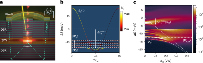
The acousto-polaritonic device studied here (Fig. 1a) is based on a patterned hybrid phonon–photon AlGaAs MC with multiple GaAs QWs placed within the spacer region between two distributed Bragg reflectors30. The distributed Bragg reflectors and the spacer are engineered to maximize the overlap between the strain field of electrically excited 7-GHz phonon and the optical 370-THz (~1,500 meV) photon modes at the QW positions. Both photonic and phononic states are vertically and laterally confined within a few-micrometre-wide thicker region of the MC spacer (simply, a trap). At 10 K, the strong coupling between QW excitons and the confined photon states leads to the formation of zero-dimensional polariton states36. We present results for a 4 × 4 μm2 trap with photon–exciton detuning of approximately −13 meV. A ring-shaped BAwR fabricated around the trap excites a fM = 7 GHz acoustic strain field polarized along the cavity growth axis. The strain couples predominantly to the excitonic polariton component via the deformation potential leading to peak energy modulation amplitudes that can exceed 25 meV (ref. 27). A detailed description of the MC sample can be found in Methods.
Figure 1b shows the time evolution of the confined states as calculated by the model to be discussed later. For clarity, only the bare exciton and the lowest five confined photonic modes are shown. The reference energy for the vertical axis corresponds to the unstrained bare exciton energy, \({E}_{{\rm{X}}}^{* }\). The latter is harmonically modulated by the strain, that is, \({E}_{{\rm{X}}}(t)={E}_{{\rm{X}}}^{* }+\Delta {E}_{{\rm{X}}}(t)={E}_{{\rm{X}}}^{* }+{E}_{{\rm{M}}}\cos ({\varOmega }_{{\rm{M}}}t)\), where ΩM = 2πfM. The energy modulation amplitude, EM, is proportional to the acoustic strain amplitude. At zero time, the exciton is well above the photonic states: ΔEX(0) ≫ ℏΩR, where ℏΩR is the light–matter Rabi coupling. Hence, the lower-energy polariton modes are photon-like. With increasing tensile strain, the bare exciton red-shifts and consecutively anti-crosses with multiple confined photonic modes. During the second half of the acoustic cycle, QWs are compressed and the bare exciton shift is reversed.
Figure 1c shows the dependence of the time-integrated photoluminescence (PL) spectrum of a trap under an excitation power below the condensation threshold (Pexc < Pth) on the acoustic amplitude (AM). The latter is proportional to the square root of the nominal radio-frequency power applied to the BAwR at ~7 GHz frequency. For AM = 0, the emission is dominated by the PL, line red-shifted by 3 meV, corresponding to the trap barrier, which is also a polariton state36. The weaker lines at lower energies are the confined polariton modes. Increasing AM spectrally broadens the level emission with the GS (\(\left|{\varPsi }_{{\rm{0}}}\right\rangle\)) broadening exceeding 10 meV for AM > 0.4. In the time-integrated spectra, this broadening arises from the time evolution of the states illustrated in Fig. 1b. Using the procedure described in Supplementary Section 2, we show that the bare exciton crosses the bare photonic GS \(\left|{\varPsi }_{\mathrm{C,0}}\right\rangle\) for AM ≈ 0.25, as indicated by the dashed lines in Fig. 1c.
We now consider the acoustic modulation in the condensation regime, that is, Pexc > Pth, which is depicted in Fig. 2a. The large spot size of the non-resonant laser relative to the trap size ensures a good spatial overlap between the reservoir and the confined polariton modes, which leads to the simultaneous population of several levels. In the absence of acoustic excitation, we observe an MMC with multiple confined polariton modes competing for the gain12. Above Pth, only the four lower levels contribute substantially to the emission. The emission of \(\left|{\varPsi }_{0}\right\rangle\) is about 30 times smaller than \(\left|{\varPsi }_{2}\right\rangle\). The excitation power dependence of the PL is discussed in Supplementary Section 3.
Fig. 2: Modulation-induced population transfer and coherence.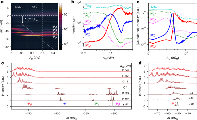
a, Experimental dependence of the trap PL on the acoustic modulation amplitude, AM, recorded for an optical excitation power Pexc ≈ 1.7Pth above the condensation threshold (Pth). The lowest energy modes are denoted by \(\left|{\varPsi }_{i}\right\rangle\). The regimes of non-equilibrium lasing (MMC) and single-mode GS condensation (GSC) are indicated. The diagonal dash-dotted line indicates the maximum excursion of the bare exciton energy, \(\Delta {E}_{{\rm{X}}}^{\max }({A}_{{\rm{M}}})\), obtained from Fig. 1c. The energy scale is referenced to the unmodulated exciton (horizontal dashed line at 0 meV). The colour bar indicates emission intensity in arbitrary units. b, Experimental time-integrated PL of the polariton states together with the total PL (labelled in the panel) determined from a as a function of AM. c, High-resolution PL spectra of the trap for several AM, recorded under conditions similar to a. The spectra are normalized in amplitude and vertically shifted for clarity. The energy scale is relative to the bare exciton energy (see a) and normalized to the modulation quantum ℏΩM = 28.7 μeV. The sharp comb peaks are phonon sidebands displaced by ℏΩM resulting from the modulation of the GS (i = 0) and of the first three excited states (i = 1, 2, 3), \(\left|{\varPsi }_{i}\right\rangle\). d, The same as c, but expanded over an energy range around GS centred at ΔE/(ℏΩM) = − 449. e, Simulated PL intensities as a function of AM for the experimental conditions in a.
The first striking observation from Fig. 2a is that, as AM increases and the levels broaden in energy, the overall PL intensity gradually shifts towards \(\left|{\varPsi }_{0}\right\rangle\). The dependence of the integrated PL intensities from confined levels on AM is summarized in Fig. 2b. The higher excited states \(\left|{\varPsi }_{2}\right\rangle\) and \(\left|{\varPsi }_{3}\right\rangle\), which dominate the emission at low AM, start to be depleted when AM ≈ 0.05 and AM ≈ 0.065, respectively. By contrast, the PL intensities from \(\left|{\varPsi }_{1}\right\rangle\) and \(\left|{\varPsi }_{0}\right\rangle\) increase until they reach a maximum at AM ≈ 0.1 and AM ≈ 0.25, respectively.
The second notable observation is the onset of an essentially single-mode condensation regime when the maximum bare exciton red-shift (diagonal dash-dotted line) approaches that of \(\left|{\varPsi }_{0}\right\rangle\) (that is, in the range 0.15 < AM < 0.3 in Fig. 2a,b). In this regime, PL becomes dominated by \(\left|{\varPsi }_{0}\right\rangle\). For AM ≈ 0.25, the \(\left|{\varPsi }_{0}\right\rangle\) PL exceeds the one from the other levels by at least an order of magnitude, thus proving a very selective particle transfer directly to the GS. When AM > 0.35, there is a partial recovery of MMC with level intensity and spectral profiles becoming weakly dependent on AM. A similar evolution of PL with AM has also been observed for other excitation powers (Supplementary Section 4).
The total PL intensity integrated over all levels (Fig. 2b, light-blue line) remains approximately constant over the whole AM range. Hence, the acoustic modulation essentially redistributes polaritons among the levels; that is, the tunable acoustic amplitude allows control over the condensation pathway to a particular level.
Despite the large energy modulation amplitudes, the high temporal coherence of the confined condensate is maintained over a wide AM range, as demonstrated by the high-resolution PL spectra of Fig. 2c, which were recorded under conditions similar to Fig. 2a using the set-up described in Supplementary Section 5. In the absence of the acoustic field, the PL consists of spectrally narrow peaks (linewidth γcond. < ΩM). The modulation induces the formation of a frequency comb of modulation sidebands separated by ℏΩM around the unperturbed condensates. The number of sidebands in each \(\left|{\varPsi }_{{i}}\right\rangle\) comb increases with AM. For small AM, the intensity of sidebands follows a Bessel distribution37, which is symmetric relative to the unmodulated resonance. For moderate and high AM, the comb spectral shape becomes strongly asymmetric. At the intermediate AM, several frequency combs are simultaneously present, indicating the Floquet nature of the modulation. The GS, \(\left|{\varPsi }_{0}\right\rangle\), emission is very weak for AM < 0.06 but dominates for AM > 0.1. As detailed in Supplementary Section 6, the spectral width of the individual lines of \(\left|{\varPsi }_{0}\right\rangle\) comb in Fig. 2d initially decreases with AM from ~0.7ℏΩM(AM = 0) to ~0.3ℏΩM(AM = 0.1) and then increases again to ~0.7ℏΩM at AM = 0.59. This behaviour correlates with the increase of the \(\left|{\varPsi }_{0}\right\rangle\) intensity followed by its reduction, which can be due to interactions with the continuum of electronic states above the bare exciton energy.
We now address the time dynamics of the polariton system via studies of the first-order auto-correlation function (∣g(1)∣) as a function of time delay (τ) using an interferometric set-up (Supplementary Section 7). The experiments were performed under a strong acoustic modulation (AM = 0.56) and Pexc ≈ 4Pth yielding the PL spectrum for the GS displayed in Fig. 3a. In addition to the modulation frequency comb, the sidebands show a clear bunching with a spacing δEbunch ≈ 5ℏΩM. Figure 3b displays the corresponding ∣g(1)(τ)∣ profile obtained by filtering the emission within the energy range indicated by the yellow background in Fig. 3a. The ∣g(1)(τ)∣ shows clear peaks at ±TM = 2π/ΩM, thus demonstrating that the \(\left|{\varPsi }_{0}\right\rangle\) coherence persists over several acoustic modulation periods. By contrast, the modulation sidebands are not resolved for the excited state, which is weakly populated: accordingly, its ∣g(1)(τ)∣ only shows a single peak at zero time delay (Supplementary Section 8). Furthermore, the GS profile has satellites at delays τsat = ± 0.2 × TM around the main peaks at 0, ±1 × TM, which correlate with the bunching of sidebands in Fig. 3a, that is, ∣τsat∣ = 2πℏ/δEbunch. The narrow temporal width, triangular shape of ∣g(1)∣ peaks and bunching provide an indirect evidence of the pulsed character of the emission, as will be elucidated by the model below.
Fig. 3: Condensate pulsing under the acoustic modulation.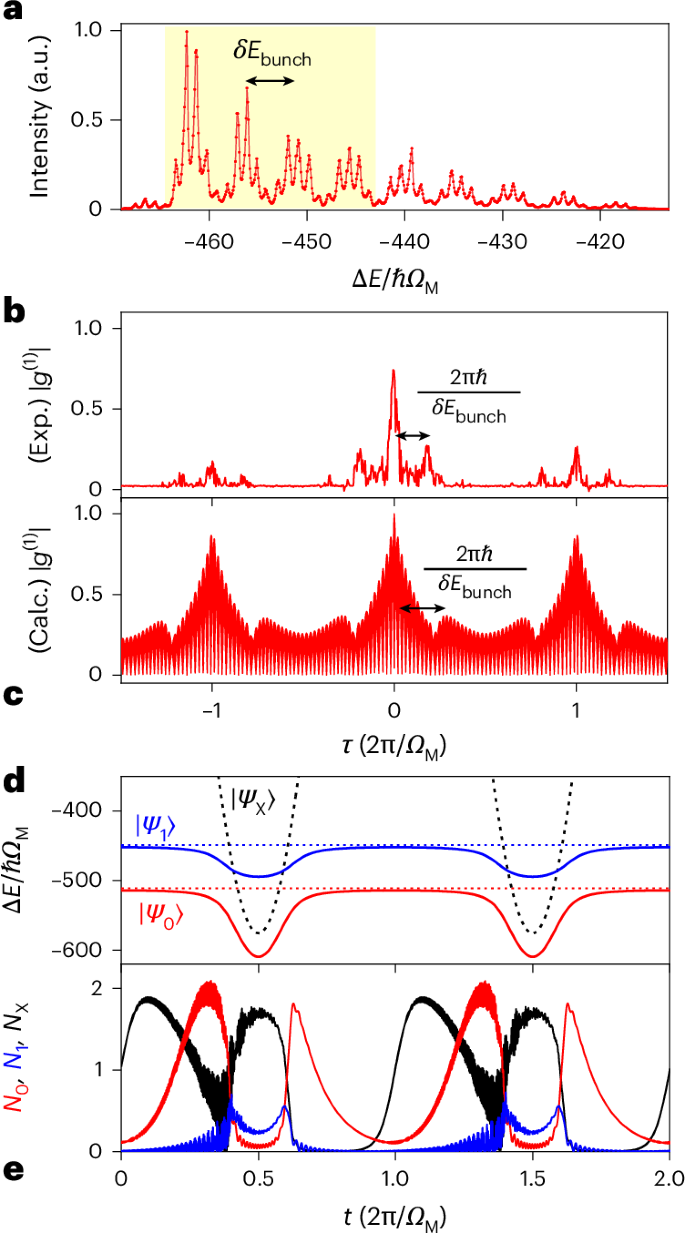
a, High-resolution PL spectrum of the GS (\(\left|{\varPsi }_{{0}}\right\rangle\)) recorded for \({A}_{{\rm{M}}}=0.59\,\sqrt{W}\). The energy scale is referenced to the bare exciton energy and normalized to the modulation quantum ℏΩM. The sideband bunching period is denoted δEbunch. b,c, First-order auto-correlation function for the GS, ∣g(1)(τ)∣ as a function of the delay τ, as determined from the visibility of the ∣g(1)(τ)∣ fringes in the energy range marked in a by the yellow rectangle the experimental (exp.) ∣g(1)(τ)∣ (b), and the calculated (calc.) ∣g(1)(τ)∣ (c). d, Simulated time evolution of the energies of the bare exciton (\(\left|{\varPsi }_{{\rm{X}}}\right\rangle\), black) and polariton GS (\(\left|{\varPsi }_{0}\right\rangle\), red) and first excited (\(\left|{\varPsi }_{1}\right\rangle\), blue) states in the steady-state regime. The dashed horizontal lines show the energies of the bare photonic levels. e, Corresponding evolutions of the steady-state level populations of the bare exciton (NX, black) as well as of the ground (N0, red) and first excited (N1, blue) bare photon states for the modulation conditions in d. The N1 population has been scaled by a factor of 10 for better visibility.
A theoretical model was developed based on the following three main assumptions (see Supplementary Section 9 for an in-depth discussion): (1) The strain field only modulates the bare exciton state, which is populated by the non-resonant optical excitation. (2) The bare exciton state feeds the polariton modes through both stimulated scattering and resonant injection due to the strong light–matter coupling. Under the acoustic modulation, the latter gives rise to a very efficient adiabatic Landau–Zener-like transfer. (3) When the bare exciton energy is shifted below the corresponding bare photonic state, the scattering from the exciton to the state becomes notably less probable and, at the same time, the losses are increased due to the overlap with the continuum of higher-energy exciton states. These processes are incorporated into an effective Gross–Pitaevskii Hamiltonian describing the coupling between exciton and photon modes given by
$$\begin{array}{l}i\hslash\displaystyle\frac{{\rm{d}}{\widetilde{\psi }}_{{\rm{X}}}}{{\rm{d}}t}=\left[{\varepsilon }_{{\rm{X}}}+{A}_{{\rm{M}}}\cos \left({\varOmega }_{{\rm{M}}}t\right)\right]{\widetilde{\psi }}_{{\rm{X}}}-\mathop{\sum }\limits_{j=1}^{n}{J}_{j}{\widetilde{\psi }}_{{\rm{C}},\,j}\\\qquad\qquad+\,\displaystyle\frac{i\hslash {\gamma }_{{\rm{X}}}}{2}\left(\widetilde{P}-{\alpha }_{{\rm{X}}}{\widetilde{n}}_{{\rm{X}}}-\mathop{\sum }\limits_{j=1}^{n}{\alpha }_{j}{\widetilde{n}}_{{\rm{C}},\,j}\right){\widetilde{\psi }}_{{\rm{X}}},\end{array}$$
(1)
$$i\hslash \frac{{\rm{d}}{\widetilde{\psi }}_{{\rm{C}},\,j}}{{\rm{d}}t}={\varepsilon }_{{\rm{C}},\,j}{\widetilde{\psi }}_{{\rm{C}},\,j}-{J}_{j}{\widetilde{\psi }}_{{\rm{X}}}+\frac{i\hslash }{2}\left({\gamma }_{{\rm{X}}}{\alpha }_{j}{\widetilde{n}}_{{\rm{X}}}-{\gamma }_{{\rm{C}},\,j}\right){\widetilde{\psi }}_{{\rm{C}},\,j}\,.$$
(2)
Equation (1) models the dynamics of the bare exciton state, ψX. The symbols with the tilde are rescaled variables introduced in Supplementary Section 9B. The first term on the right-hand side of the equation represents the exciton energy, εX, modulated by the time-dependent strain. The second term accounts for the coherent light–matter coupling between the exciton and the bare confined photon states, ψC,j (j = 0, 1, …, n − 1), where n is the total number of confined photonic states, leading to the formation of polaritons. The strength of this coupling is characterized by the Rabi coupling energy Jj = ℏΩR,j, which governs the rate of population exchange between the exciton and each confined state. Finally, the third term accounts for the non-Hermitian nature of the system in the condensation regime. Here, \(\widetilde{P}\) represents the net injection rate of particles into the exciton state state (relative to the level at the condensation threshold) from the optically non-resonantly pumped reservoir, while γX denotes the exciton decay rate. The term \({\alpha }_{{\rm{X}}}{\widetilde{n}}_{{\rm{X}}}\) describes exciton saturation effects, where αX is the filling rate constant, and \({\widetilde{n}}_{{\rm{X}}}={\left|{\widetilde{\psi }}_{{\rm{X}}}\right|}^{2}\) is the exciton density. Finally, \({\sum }_{j=1}^{n}{\alpha }_{j}{\widetilde{n}}_{{\rm{C}},j}\) represents the total stimulated scattering rate into the confined photonic states, where αj is the filling rate constant for each state and \({\widetilde{n}}_{{\rm{C}},j}={\left|{\widetilde{\psi }}_{{\rm{C}},j}\right|}^{2}\) is the corresponding density.
Similarly, equation (2) describes the dynamics of the confined light modes. The first term on the right-hand side corresponds to their bare energies εC,j, which depend on the lateral confinement potential. The second term accounts for the light–matter interaction with the exciton state. The third term describes the filling of the confined states through stimulated scattering from the exciton at a rate \(\gamma {\alpha }_{j}{\widetilde{n}}_{{\rm{X}}}\) as well as their dissipation due to cavity losses with a decay rate γj. The losses depend on the detuning of between the exciton and photonic modes and, thus, on time, as discussed in Supplementary Section 9C. The parameters used in the simulations are listed in Supplementary Section 9D.
The dependence of time-averaged populations of the different levels as predicted by the model is shown in Fig. 2e. The predictions excellently reproduce the progressive loading of the levels shown in Fig. 2b. Figure 3d,e shows, respectively, the simulated time evolution of the energies and populations of the bare exciton (\({\widetilde{n}}_{{\rm{X}}}=| \left\langle {\psi }_{{\rm{X}}}\right\rangle {| }^{2}\)), ground (\(\widetilde{{n}_{0}}=| \left\langle {\psi }_{{\rm{C}},0}\right\rangle {| }^{2}\)) and first excited (\(\widetilde{{n}_{1}}=| \left\langle {\psi }_{{\rm{C}},1}\right\rangle {| }^{2}\)) polariton states in the steady-state regime. The short-time transient after the modulation turn-on is discussed in Supplementary Section 10. The configuration of energy levels as well as the optical and acoustic excitation correspond approximately to the conditions of Fig. 2a for AM ≈ 0.25. The population data of Fig. 3e are also represented in an alternative way by the colour lines in Fig. 1b.
We consider the evolution of the populations during the modulation cycle of Fig. 3e. For a large negative dynamic detuning between the bare exciton and the photonic GS, \({\delta }_{{{\rm{C}}}_{0}-{\rm{X}}}(t=0)\ll 0\), the exciton holds most of the population and photonic levels are essentially empty. As \({\delta }_{{{\rm{C}}}_{0}-{\rm{X}}}(t)\) reduces, the higher levels become progressively more populated, while the exciton is depopulated. For each level, the maximum population is achieved very close to the respective avoided crossing point, where the population transfer is due to the coherent Rabi oscillations.
As the exciton moves below a photonic level \(\left|{\varPsi }_{{\rm{C}},j}\right\rangle\), this level becomes depopulated. Below \(\left|{\varPsi }_{{\rm{C}},0}\right\rangle\), the stimulated scattering mechanism is suppressed and there is a partial recovery of the exciton population. As the exciton approaches \(\left|{\varPsi }_{{\rm{C}},0}\right\rangle\) from below, there is a fast Rabi transfer of the population, which leads to the second emission pulse at t = 0.65(2π/ΩM) in Fig. 3e. The time separation between the subpulses depends on the modulation amplitude. For \(\left|{\varPsi }_{C,0}\right\rangle\) crossing conditions, the subpulsing frequency is approximately 2 × ΩM/2π.
The \(\left|{\varPsi }_{C,0}\right\rangle\) time evolution of Fig. 3e leads to the ∣g(1)∣ shown in Fig. 3c (the corresponding comb spectrum is discussed in Supplementary Section 11). The triangular shape of the pulses gives rise to the triangular shape of ∣g(1)∣, while the pulsing leads to the additional peaks at ±TM = 2π/ΩM and the features displaced by 2πℏ/δEbunch associated with the subpulsing—the cause of the spectral bunching of sidebands. The good agreement between the measured and simulated auto-correlation functions displayed in Fig. 3b,c, respectively, confirms the validity of the modelled time evolution.