
Reforestation potential maps
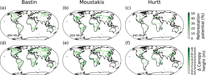
This study analyzes the climate response to three distinct reforestation potentials, focusing on their impact on temperature. Our literature review identified 19 global maps for reforestation4,13,14,15,16,17,18,19,20,21,22,23,24,25,26,27,28,29,30. From these, we selected the datasets by Bastin et al.15, Moustakis et al.24, and Hurtt et al.18 for implementation in our simulations (hereafter referred to as Bastin, Moustakis, and Hurtt reforestation potentials). The Bastin et al.15 reforestation potential is based on satellite and ground-based measurements combined with machine learning. The Moustakis et al.24 map was chosen for its integrated approach, which synthesizes thousands of Integrated Assessment Model (IAM) scenarios with existing reforestation datasets from Griscom et al.4 and the Atlas of Forest Landscape Restoration Opportunities (FLRO13), offering a more synthesized and policy-relevant perspective. Both the maps by Bastin et al.15 and Moustakis et al.24 serve as an upper-bound estimate of global reforestation potential (935 Mha for Moustakis and 900 Mha for Bastin), which is useful to estimate the maximum potential effect that large-scale reforestation could have. The Bastin reforestation potential has drawn notable criticism, including for its widespread reforestation in boreal regions that likely induces BGP warming33,58. The geographic differences between our two scenarios, therefore, allow for a comparative analysis of the climate impacts of reforestation placement and provide a means to evaluate some of these previously raised concerns. Lastly, we selected the SSP1-2.6 scenario from Hurtt et al.18. This scenario is a component of the Land-Use Harmonization version 2 (LUH2) dataset, which is a standard input for climate models, and is derived from the Integrated Assessment Model IMAGE that includes a dynamic vegetation model. The Hurtt reforestation scenario thus serves as an important bridge between established climate community land-use scenarios and the recent ecology- or machine learning-based reforestation potentials. Additionally, we selected this SSP1-2.6 land-use scenario as it is a low warming scenario that is close to the Paris Agreement and represents a medium reforestation potential (around 440 Mha) compared to the other two datasets. Note that the difference in SSPs used for the forcing (SSP2-4.5) and the Hurtt reforestation potential (SSP1-2.6) will not cause any inconsistencies, as we are investigating the climate response to a land-use perturbation, not the socio-economic feasibility of achieving this change in land-use within the SSP2-4.5 world. Table S1 provides detailed information on the methodologies, underlying assumptions, total reforestation area, total carbon uptake, and climatic context for these three selected reforestation potentials15,18,24.
Other available reforestation potential maps were not selected due to several limiting factors, including practical feasibility, assumed safeguards and availability. Some datasets14,19,27 assumed an unrealistic absence of human activity, proposing reforestation across all cropland and cultivated grassland areas. Moreover, the dataset by Laestadius et al.13 has been critiqued for potentially overestimating the global reforestation potential. A key technical consideration was the unit of measurement: several potential restoration datasets14,17,19,22,23,30 were provided in units of carbon uptake. This would have necessitated a complex conversion from carbon to a suitable forest input map for CESM2. Furthermore, some datasets16,20,25 did not have openly available data repositories, and others did not provide estimates at the gridcell level21. Additionally, the Griscom et al.4 was not chosen as it is considered in the Moustakis et al.24 dataset and the Weber et al.26 dataset as it has already been implemented in CESM2. The recent datasets from Fesenmyer et al.28 and Roebroeck et al.29 were published after the completion of our simulations. While the dataset from Fesenmyer et al.28 would be valuable for future climate model implementations to represent a lower-bound estimate, exploring such a scenario would require substantial additional computational resources. This is because the resulting weak climate signal, stemming from the small restoration area, would require a larger ensemble size to be reliably separated from natural climate variability.
Implementation of reforestation potential maps
To assess the impact of future reforestation scenarios on the climate, we conducted simulations based on reforestation potentials by Bastin et al.15, Moustakis et al.24, and Hurtt et al.18 in comparison to a baseline scenario under SSP2-4.5 forcing. In the baseline scenario, land cover (natural vegetation and cropland) was held constant at the 2015 level for the entire length of the simulation (2015 to 2100).
We then generated a land-use timeseries input for the Community Land Model version 5 (CLM5), the land component of CESM241, based on the three different reforestation potentials. For the Bastin dataset, we used the reforestation potential rather than the global potential tree cover to avoid the impact of differing climatological tree cover distribution based on satellite- and ground-based data from Bastin et al.15 and CLM5. We then followed these steps to generate a land-use timeseries input for CLM5 based on the Bastin reforestation potential: First, we converted the Bastin et al.15 reforestation potential from the original TIFF format into a NetCDF file. The Bastin dataset assumes that grid cells with non-zero reforestation potential are set to 100% land cover, while regions with zero potential or ocean areas contain not-a-number (NaN) values. For integration into CLM5, remapping to the CESM2 resolution necessitated accounting for changes in land fraction. This was achieved by employing the Bastin future risk data (which includes NaN values over oceans and numerical values over land) to construct a land-ocean mask. Applying this mask to the Bastin reforestation potential data preserved NaN values over the ocean, introduced zeroes for land areas with no reforestation potential, and maintained the original reforestation values in all other land grid cells. Next, we conservatively remapped the Bastin dataset from its native resolution (30 arc sec) to the CESM2 resolution of 0.9° latitude × 1.25° longitude. This yielded a land-specific map of Bastin data at CESM2 resolution, to which we applied the CESM2 land-sea mask, ensuring that non-zero reforestation potential was assigned exclusively to land areas within CESM2.
To create a Moustakis input dataset, we used the change in forest fraction data in 2100 at the grid cell level24. This data contains NaN values over the ocean and values ranging from 0 to 1 reforestation potential over land, expressed as fractions of grid cell area. We divided this potential by the land fraction of MPI to get land-specific values. We then conservatively remapped the data to the resolution of CESM2 and masked the remapped dataset by the land-sea mask from CESM2.
As the third dataset, we created a reforestation potential input file based on the SSP1-2.6 scenario from Hurtt et al.18. For this, we used the SSP input for the CESM2 model (which is already at CESM2 resolution) and converted the forest cover data to land-specific values. We then calculated the maximum forest cover in every grid cell from 2015 to 2100 to define a reforestation potential. This approach of using the maximum forest cover across the time period, rather than the difference between forest cover in 2100 and 2015, ensured that only reforestation (and no deforestation) was implemented, thereby making this definition of reforestation potential more comparable across datasets.
After creating CLM-resolution maps for all three reforestation potentials, we constructed a land-use timeseries file for CLM5. For this, we calculated a linear reforestation trajectory from 2015 to 2070 for each gridcell, ensuring that the full reforestation potential for each gridcell of each respective dataset was attained by 2070. This method accounts for regional variations in reforestation speed due to unique linear trajectories for each gridcell, reflecting the likely heterogeneous reforestation efforts. To accommodate reforestation, existing vegetation types were removed hierarchically in the following order: shrubs (PFTs 9-11), grasses (PFTs 12-14), and then crops (CFTs) (Fig. S6). This specific hierarchy was chosen to minimize the reduction of non-irrigated and irrigated cropland. Note that it is assumed that no future expansion of croplands or grazing lands occurs according to our implementation, which could be attributed to shifts in dietary patterns or increased efficiency in existing agricultural practices. Additionally, bare soil, ice-covered regions and urban areas were excluded from reforestation to maintain consistency with the safeguards applied in the reforestation potentials and considering the small likelihood of plant growth in bare soil and ice-covered regions. After the fraction of shrub, grass and cropland was reduced, the original forest fraction is scaled up proportionally to match the projected reforestation potential in that grid cell. Note that reforestation was only implemented in regions where CESM2 already contained forest. In locations where a reforestation potential dataset suggested reforestation but CESM2 did not contain forest historically (i.e., in 2015), land cover was reverted to its original distribution, although adjustment impacted only less than 1% of the grid cells. To investigate equilibration effects after the full forest change is implemented, we extended the simulations beyond 2070 by maintaining full reforestation potential for an additional 30 years, until 2100.
Using this methodology, we successfully implemented around 99% of the Bastin reforestation potential into CESM2. The remaining 1% could not be incorporated due to geographic constraints, as these areas—primarily located in the Canadian Arctic, parts of Greenland and Siberia—were either covered by snow and ice, classified as urban or bare soil, or already fully forested in CESM2. Similarly, we were able to implement over 99% of the Moustakis and Hurtt scenario (Table S1).
CESM2 model and experimental design
The simulations in this study were performed with the fully-coupled CESM2.1.2 model to capture forest-induced climate response and allow an examination of coupled biosphere-atmosphere-ocean interactions. Previous research has demonstrated robust model performance of CESM2 concerning Leaf Area Index (LAI) sensitivity, albedo, and surface radiation39, as well as in simulating temperature and precipitation patterns59. The model has a horizontal resolution of 0.9° latitude × 1.25° longitude and comprises the Community Atmospheric Model version 6 (CAM6), the Community Land Model version 5 (CLM5), the Parallel Ocean Program version 2 (POP2), the Los Alamos Sea Ice Model (CICE), the Model for Scale Adaptive River Transport (MOSART) and the Land Ice Model (CISM2). The CESM2 model version used here does not allow dynamic changes in vegetation composition. We used the biogeochemical (BGC-Crop) mode in CLM5, as it includes active biogeochemistry and fires, and provides a more physically plausible representation of vegetation dynamics by allowing trees to die if planted outside their suitable climatic regions49.
Each simulation was run from 2015 to 2100 in a concentration-driven mode, driven by the transient forcing of SSP2-4.5 (BSSP245cmip6 compset) with the exception of land use change. In the control simulation, forest cover was held constant at 2015 levels. In the three reforestation simulations, the reforestation potential from Bastin, Moustakis, and Hurtt was linearly increased from 2015 to 2070, followed by 30 years of constant forest cover. Land-use options such as harvesting, grazing, and nitrogen fertilizer usage were set to zero in the control and reforestation simulations, while irrigation could dynamically respond to simulated soil moisture conditions.
To reduce the effect of internal variability and enhance the signal-to-noise ratio, five ensemble members were run for both the control and each reforestation potential simulation. These ensemble members branched off from 2015 from the BHISTcmip6 simulations of the CESM2 Large Ensemble (CESM2-LE60). We excluded the BSMBB simulations due to the limited availability of restart files and to maintain consistency with CMIP6 historical simulations. The selection of CESM2-LE ensemble members was based on latitude-weighted sea surface temperatures (SSTs) over the subpolar North Atlantic (SPNA) region (45-65°N, 50°W-0°), averaged over 2010-2014. This index is strongly correlated with the strength of the Atlantic Meridional Overturning Circulation (AMOC)61. Specifically, we chose ensemble members that fell within the 10th, 25th, 50th, 75th and 90th percentiles of the SPNA SST distribution, corresponding to weak (ensemble members 1251.010), medium-weak (ensemble member 1141.008), medium (ensemble member 1251.005), medium-strong (ensemble members 1281.009) and strong (ensemble member 1021.002) AMOC states, respectively. This approach allows for an assessment of the sensitivity of our results to underlying patterns of oceanic variability while ensuring that the simulations encompass a broad range of possible initial conditions.
The results are presented as the ensemble means, which represent the biogeophysical effects of global reforestation driven by changes in albedo, evapotranspiration and surface roughness. To calculate the ensemble means, we first calculate the difference of each reforestation potential ensemble member from the according baseline ensemble member (Fig. S7) and then take the ensemble mean. We present ensemble means to reduce the influence of internal variability, and because the influence of the AMOC initialisation state on the simulated response diminished rapidly, becoming negligible beyond the initial 20 years of simulations. The analysis focused on near-surface air temperature changes. This temperature variable is defined as 2 m above the combined roughness length and displacement height, meaning that the temperature usually lies above the tree canopy in forested areas. CESM2 (and other ESMs) does not have a temperature variable that would capture surface shading effects from trees, which would lead to local cooling effects just below the tree canopy. All spatial maps are shown as a time average over the last 30 years of the simulation (2071–2100), during which forest cover was held constant. The significance of the results has been evaluated using a two-sample t-test with Benjamini-Hochberg correction62,63. Stippling in spatial figures shows significant responses at the 90% significance level.
Calculation of the biogeochemical temperature effect of reforestation
Since our simulations are concentration-driven and solely capture the biogeophysical effects of reforestation, we approximate the associated biogeochemical temperature effect based on changes in land carbon stocks. This approximation uses the concept of the transient climate response to cumulative emissions (TCRE)42,51,64. The TCRE quantifies the amount of global warming per unit of cumulative fossil fuel emission at the point of doubling of atmospheric CO2 concentration relative to a baseline. A key characteristic of the TCRE is its approximate constancy over time and independence from the specific emission trajectory65. To estimate the global-mean near-surface temperature change attributable to the biogeochemical impacts of reforestation (\(\Delta {\bar{T}}_{{{\mathrm{BGC}}}}\)), we use the following formula from Amali et al.42:
$$\Delta {\bar{T}}_{{{\mathrm{BGC}}}}=-{{{\mathrm{TCRE}}}}\cdot \Delta {\bar{C}}_{{{\mathrm{Land}}}}$$
(1)
where \(\Delta {\bar{C}}_{{{\mathrm{Land}}}}\) represents the total change in the land carbon stock (variable TOTECOSYSC from CESM2) between the baseline and each reforestation scenario and the TCRE value of 2.13 °C EgC−1 for the CESM2 model is taken from Arora et al.43. The overbars denote global-mean values. We additionally did a sensitivity test by repeating the calculations with TCRE values based on the observational range identified by the IPCC AR6 (1.0–2.3 °C EgC−1 with a best estimate of 1.65 °C EgC−152) and the CMIP6 ESM range (1.32–2.3 °C EgC−143), with the results presented in Fig. S5 and described in the discussion section.
Separation of local and nonlocal signals using Moving Window Regression
We disentangled the local and non-local biogeophysical temperature responses to identify regions that could directly benefit from reforestation versus those primarily influenced by remote climate signals. Local responses arise from in-situ land-atmosphere interactions due to changes in surface properties like roughness, evaporative capacity, and albedo66. Non-local responses are remotely induced by larger-scale atmospheric or oceanic changes. This separation provides a deeper understanding of the interplay between local surface processes and the large-scale climate system.
Here, we used the MWR method67,68. This method has been proven effective in extracting the LULCC signal from simulations [e.g., ref. 66] and observations [e.g., ref. 69]. For each grid cell, a linear regression is performed between the near-surface temperature change (climate response) and tree cover fraction change (surface forcing) across surrounding grid cells within a defined window. The intercept of this linear regression represents the non-local signal, which is the climate response that would be present without LULCC in the specific grid cell and is influenced by atmospheric processes. The slope of the regression gives the local signal, which is assumed to be directly related to land cover changes within the grid cell. The total response is then calculated as the sum of the local and non-local signal. The MWR method has proven to provide estimates of local versus non-local temperature responses compatible with estimates from other methods like checkerboard interpolation and spectral decomposition70.
In this study, we used a 9 × 9 grid cell window for the MWR. Consistent with previous literature70, we found that the results are largely insensitive to the window size. Thus, we chose a 9 × 9 window which provides a suitable trade-off between capturing significant trends and accurately explaining the simulated behaviour.