
Optical setup
The optical setup is shown in Extended Data Fig. 1. Light emitted by an infrared fibre laser (NKT Photonics Koheras Adjustik E15) passes through the fibre electro-optic modulator EOM 2. We split off a small fraction of the light to lock the cavity (Extended Data Fig. 1a). The rest is amplified to a power of 6 W (NKT Photonics Boostik HP) and then divided into three parts: one for phase-noise detection, one serving as the LO in heterodyne detection (Extended Data Fig. 1c) and up to 3 W for the optical tweezer.
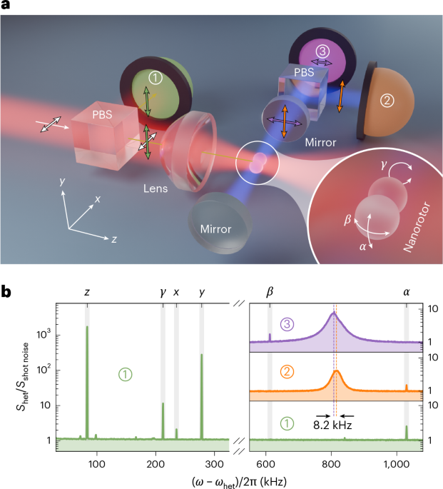
The tweezer mode is cleaned by a polarization-maintaining fibre, and its polarization is set by wave plates to be linear along the cavity axis. This orientation minimizes Rayleigh scattering into the cavity when the nanorotors are perfectly aligned. The laser light fills the aspherical tweezer lens, which has a diameter of 25.4 mm, a numerical aperture of numerical aperture of 0.81 and an effective focal length of 13.2 mm (Thorlabs, custom design). For a cluster assembled using 119-nm nanospheres (Fig. 1b), we determine a trap power of P = 2.7 W and trapping waists of wx = 1.17 μm and wy = 0.98 μm.
We detect the trapped nanoparticle by collecting its backscattered light (Extended Data Fig. 1c). Its two polarization components are split by the PBS and detected separately. The vertical component provides the most information about the particle’s rotation, particularly about the rotation around the tweezer propagation axis z. This signal is only weakly sensitive to Rayleigh scattering of the aligned rotor and scattering at surfaces along the beam path. Therefore, this component is used to monitor cooling to the librational ground state. The horizontal contribution is isolated using a fibre circulator, which provides intrinsic alignment of the backscattering signal and is, therefore, used during trap alignment. To reduce the Rayleigh scattering peak, we filter the electrical signal using a crystal oscillator.
The trapped nanoparticle is centred at an antinode of the cooling cavity mode. The resonator is formed using mirrors with intensity reflectivity of R ≥ 0.99999 (FiveNine Optics) and radius of curvature of 5 cm, yielding a finesse of \({\mathcal{F}}\approx300,000\) at a free spectral range of 9.72 GHz, corresponding to a linewidth of κ/2π = 32.4 kHz and a central waist of wcav = 94 μm. By careful design of the cavity mirror mount (Extended Data Fig. 4), we achieve an alignment of the cavity modes both along and orthogonal to the direction of tweezer propagation. The birefringence splitting between the two modes can be tuned in the range of 2π × (0−30 kHz) by applying pressure onto the mirrors via screws.
We lock the laser to the cavity using the Pound–Drever–Hall scheme (Extended Data Fig. 1a). EOM 1 (iXblue, PHT MPZ-LN-10-00-P-P-FA-FA) generates the locking sidebands and is used together with acousto-optic modulator AOM 1 (G&H, T-M200-0.1C2J-3F2P) to shift the locking frequency by one free spectral range of the cavity. This minimizes interference between the locking and the cooling light in detection.
To detect the particle motion in all directions, we use a heterodyne scheme, which mixes the scattered light with an LO. This enhances the signal interferometrically and shifts the signal to a spectral range of lower noise. The LO is blueshifted by 4.99814 MHz with respect to the tweezer beam using two polarization-maintaining fibre modulators (G&H, T-M200-0.1C2J-3F2P): AOM 2 at 197.5 MHz and AOM 3 at −202.49 MHz (Extended Data Fig. 1c).
The scattered light transmitted by the cavity mirror is divided into its horizontal and vertical polarization components. They are individually combined with the LO beam using a 50:50 fibre beamsplitter (Thorlabs PN1550R5A2). Each polarization output is then detected by a balanced photodiode (Thorlabs PDB425C-AC). In both backplane detections, we use variable-ratio fibre beamsplitters (KS Photonics) to balance the outputs, which are also detected by balanced photodiodes (Thorlabs PDB440C-AC) (Extended Data Fig. 1c).
After the optical trap, we collimate the tweezer light using a low-numerical-aperture aspheric lens (Thorlabs C560TME-C) and isolate the particle signal using a split detection scheme (Extended Data Fig. 1d). We use a D-shaped mirror to split the optical beam into two halves that are detected by balanced photodiodes (Thorlabs PDB440C-AC). This detection is built for both x and y axes.
Phase-noise reduction
In the presence of the cavity, laser phase noise can heat the mechanical motion55. The cavity delays the release of scattered light, effectively creating an unbalanced interferometer in heterodyne detection between scattered light and the LO. The laser phase noise appears in cavity transmission as an increased noise background around the cavity mode resonance. In Fig. 1b, this is shown at a frequency of around ~800 kHz and fitted with a Lorentzian to extract the exact frequency and to determine the birefringence splitting. We also use the fitted frequency to determine the actual tweezer–cavity detuning and its error during the detuning scan (Fig. 2e).
Strong cooling of the librational modes without the active suppression of phase noise leads to noise squashing61 (Extended Data Fig. 2c, top), which distorts the motional sideband and generates a dip in the phase-noise background. This prevents accurate sideband thermometry. We, therefore, implement a phase-noise reduction scheme, using an unbalanced Mach–Zehnder interferometer43 (Extended Data Fig. 1b). The short arm contains a polarization-maintaining fibre attenuator to equalize the optical power in both arms. The long arm consists of a 100-m single-mode fibre (SMF-28), enclosed in a chamber at prevacuum. This arm also includes a fibre stretcher to stabilize slow path-length fluctuations (>10 ms), and it combines a manual fibre polarization controller and a fibre PBS to correct for polarization changes. Light from both arms is recombined using a 50:50 fibre coupler and directed to a balanced detector (Thorlabs PDB450C-AC). After filtering, the interferometer output is fed back into EOM 2, which controls the phase of the tweezer light.
With active feedback, the noise level is reduced by more than 30 dB both at a single frequency (Extended Data Fig. 2b) and two frequencies (Extended Data Fig. 2c, bottom). The reduction is also visible in cavity transmission, restoring the expected shape of the motional sidebands (Extended Data Fig. 2, middle).
Mode identification
To assign the peaks shown in Fig. 1b to translational and librational modes, we first use the fact that the translational frequencies for nanoparticles much smaller than the optical wavelength hardly depend on the particle shape. We, therefore, use individual spherical nanoparticles to identify the frequencies associated with the z, x and y modes, where the x and y frequencies change depending on the tweezer polarization, whereas the z frequency stays invariant. When switching to anisotropic nanoparticles, three additional frequency peaks appear. Due to the prolate geometry of our nanorotors (mostly dimers and linear trimers), we have one peak at smaller frequencies (γ) and two peaks at larger frequencies. As described in the ‘Experimental setup’ section, we use the polarization-sensitive detection of the cavity transmission to discriminate between α and β.
Theoretical description
The nanorotor is an asymmetric rigid body (Ic < Ib < Ia), whose orientation in the laboratory frame (ex, ey, ez) is specified by the three Euler angles (α, β, γ), using the z–y′–z″ convention (Fig. 1a, inset). Its optical response is characterized by the susceptibilities χa < χb < χc (ref. 42), which can be combined into the susceptibility tensor χ = χan1 ⊗ n1 + χbn2 ⊗ n2 + χcn3 ⊗ n3, where n1, n2, n3 are basis vectors. The particle is illuminated by the linearly polarized tweezer field Etw(r) = Etw(r)eϕ of wavelength 2π/k with the tweezer mode amplitude Etw(r) ∝ eikz propagating in the ez direction and the polarization direction \({{\bf{e}}}_{\phi }={{\bf{e}}}_{x}\cos \phi +{{\bf{e}}}_{y}\sin \phi\). Coherent scattering of tweezer photons couples the deeply trapped particle rotations to two orthogonally polarized modes of the cavity field Ec(r) = Ec(r)(eyay + ezaz), with \({E}_{{\rm{c}}}({\bf{r}})\propto \cos (kx)\) denoting the cavity mode amplitude and ay,z the corresponding complex mode variables. The resulting interaction potential can be derived from the Lorentz torque acting on the particle as35,36,42
$$\begin{array}{rcl}U & = & -\frac{{\varepsilon }_{0}V}{4}{{\bf{E}}}_{\mathrm{tw}}\cdot \chi {{\bf{E}}}_{\mathrm{tw}}^{* }\\ & & -\frac{{\varepsilon }_{0}V}{4}\left({{\bf{E}}}_{{\rm{c}}}\cdot \chi {{\bf{E}}}_{\mathrm{tw}}^{* }+\mathrm{h.c.}\right).\end{array}$$
(4)
Here V denotes the particle volume and R is the particle centre-of-mass position. Since the particle remains stably trapped at R ≃ 0, the first term describes the librational trapping near (α, β) ≃ (ϕ, π/2). The second term describes the coupling of librations in α and β to two orthogonally polarized cavity modes as well as trapping of γ. In our experiment, γ ≃ 0 or γ ≃ π/2 because the cavity modes are polarized along ey and ez. In the following, we assume γ ≃ π/2; the case of γ ≃ 0 can be obtained by exchanging indices a ↔ b. The librational frequencies for deviations of α and β from their equilibrium orientation are given by
$$\begin{array}{l}{\varOmega }_{\alpha }=\sqrt{\frac{{\varepsilon }_{0}V}{2{I}_{b}}({\chi }_{c}-{\chi }_{a})}| {E}_{{\rm{tw}}}(0)| ,\\ {\varOmega }_{\beta }=\sqrt{\frac{{\varepsilon }_{0}V}{2{I}_{a}}({\chi }_{c}-{\chi }_{b})}| {E}_{{\rm{tw}}}(0)| .\end{array}$$
(5)
The second term in equation (4) decomposes into an orientation-independent term that drives the in-plane cavity mode ay and an orientation-dependent term that describes coupling between the cavity modes and particle librations. Specifically, the former term can be written in the form Vdr = ℏ(ηay + h.c.) with the pump rate
$$\eta =-\frac{{\varepsilon }_{0}{\chi }_{a}V}{4\hslash }{E}_{{\rm{c}}}(0){E}_{{\rm{tw}}}^{* }(0)\sin \phi .$$
(6)
Likewise, the coupling between librations and the cavity modes follows from the orientation of the susceptibility tensor. For ϕ = 0, the coupling becomes approximately linear in both librational degrees of freedom:
$${U}_{{\rm{int}}}\approx {k}_{\alpha }\alpha {a}_{y}+{k}_{\beta }\beta {a}_{z}+{\rm{h.c.}},$$
(7)
where the complex-valued constants for both librational modes are given by
$$\begin{array}{l}{k}_{\alpha }=\frac{{\varepsilon }_{0}V}{4}({\chi }_{c}-{\chi }_{a}){E}_{{\rm{c}}}(0){E}_{\mathrm{tw}}^{* }(0),\\ {k}_{\beta }=\frac{{\varepsilon }_{0}V}{4}({\chi }_{c}-{\chi }_{b}){E}_{{\rm{c}}}(0){E}_{\mathrm{tw}}^{* }(0).\end{array}$$
(8)
For both values of γ, equation (7) shows that α couples to the in-plane cavity mode ay, whereas β couples to the out-of-plane cavity mode az. Cavity-transmission spectra (Fig. 1b) consistently show Ωα > Ωβ across all nanorotors trapped in our setup, which is compatible with γ ≃ π/2 and motivates this choice in our modelling.
We define the librational mode variables bα = αzpf(α + ipα/IαΩα) and bβ = βzpf(β − π/2 + pβ/IβΩβ), with zero-point fluctuation amplitudes \({\alpha }_{{\rm{zpf}}}=\sqrt{\hslash /2{I}_{b}{\varOmega }_{\alpha }}\) and \({\beta }_{{\rm{zpf}}}=\sqrt{\hslash /2{I}_{a}{\varOmega }_{\beta }}\), to obtain the quantized interaction Hamiltonian of equation (1), where we introduced the coupling constants
$$\begin{array}{l}{g}_{\alpha }={\alpha }_{{\rm{zpf}}}{k}_{\alpha },\\ {g}_{\beta }={\beta }_{{\rm{zpf}}}{k}_{\beta }.\end{array}$$
(9)
In summary, this leads to the total libration cavity Hamiltonian in equation (2). A standard calculation then yields the optomechanical damping rates and the resulting steady-state occupation in equation (3)42.
Optomechanical coupling
The optomechanical coupling determines the interaction between the particle and cavity mode and, therefore, the cooling performance. By solving the equations of motion, with cooling providing additional damping, we obtain an effective motional linewidth of
$${\gamma }_{\mu }^{\mathrm{eff}}(\omega )={\gamma }_{\mu }+\frac{4| {g}_{\mu }{| }^{2}{\varOmega }_{\mu }{\Delta }_{{\rm{c}}}\kappa }{\left[{\left(\frac{\kappa }{2}\right)}^{2}+{(\omega +{\Delta }_{{\rm{c}}})}^{2}\right]\left[{\left(\frac{\kappa }{2}\right)}^{2}+{(\omega -{\Delta }_{{\rm{c}}})}^{2}\right]},$$
(10)
which depends on the coupling strength. In the regime of strong cooling, when the cavity resonance is close to the mechanical frequency, energy loss through the cavity determines the damping and the cavity-induced linewidth dominates over the thermal linewidth γμ. We use this expression to fit the linewidths extracted from cavity-detuning scans for 1D (Fig. 2d) and 2D (Extended Data Fig. 3c) cooling with a constant coupling. We verify the extracted coupling by additionally fitting the observed optical spring effect (Fig. 2c):
$${\varOmega }_{\mu }^{\mathrm{eff}}(\omega )=\sqrt{{\varOmega }_{\mu }^{2}-\frac{4\,| {g}_{\mu }{| }^{2}\,{\varOmega }_{\mu }\,{\Delta }_{{\rm{c}}}\left[{\left(\frac{\kappa }{2}\right)}^{2}-{\omega }^{2}+{\Delta }_{{\rm{c}}}^{2}\right]}{\left[{\left(\frac{\kappa }{2}\right)}^{2}+{(\omega +{\Delta }_{{\rm{c}}})}^{2}\right]\left[{\left(\frac{\kappa }{2}\right)}^{2}+{(\omega -{\Delta }_{{\rm{c}}})}^{2}\right]}}.$$
(11)
Since the optomechanical coupling is determined by the rotor geometry, we can determine the moment of inertia for each mode. Combining equations (5) and (8) with the zero-point fluctuation, we calculate as follows:
$${I}_{b}=\frac{| {g}_{\alpha }{| }^{2}}{{\varOmega }_{\alpha }^{3}}\frac{| {E}_{{\rm{tw}}}(0){| }^{2}}{| {E}_{c}(0){| }^{2}8\hslash },\,{I}_{a}=\frac{| {g}_{\beta }{| }^{2}}{{\varOmega }_{\beta }^{3}}\frac{| {E}_{{\rm{tw}}}(0){| }^{2}}{| {E}_{c}(0){| }^{2}8\hslash }.$$
(12)
Noise contributions
For quantum-limited measurements, the signal must be isolated from noise. The noise contributions in backscattering detection are shown in Extended Data Fig. 2a. The raw spectrum contains dark noise (photodetector and oscilloscope), shot noise and phase noise of the LO. The latter originates from the frequency generators that drive LO AOMs 2 and 3 (Extended Data Fig. 1c). In postprocessing, we, therefore, subtract the background levels as extracted from the Lorentzian fits. Additionally, the detector sensitivity shows a weak frequency dependence, which differs for the Stokes and anti-Stokes peaks. The sensitivity is calibrated by acquiring the spectra of dark noise and LO’s shot noise. Since shot noise is white, any residual frequency dependence must be due to the detector response. We, therefore, divide the background-corrected signals by the difference between shot noise and dark noise.
Occupation number
The areas of the Stokes (AS) and anti-Stokes (AaS) peaks scale with the mean occupation number n of the harmonic oscillator as AS = C(n + 1) and AaS = Cn, respectively, where C is a proportionality constant. The occupation number can, therefore, be extracted from the ratio of the Stokes and anti-Stokes peak areas62. In practice, the precision of area measurements is limited by the available integration time. When recording a detuning scan within a fixed total acquisition time, increasing the number of detuning points necessarily reduces the integration time per point, which would, in turn, degrade the precision of the occupation number estimates. Since the difference in the sideband areas satisfies AS − AaS = C, independent of the occupation number n, we determine C by averaging the differences AS − AaS over all spectra in a given scan. Figure 2b and Extended Data Fig. 3a,b show the resulting normalized peak areas AS/C and AaS/C, whose difference is supposed to be unity by construction. The occupation number at each detuning is then obtained from n = (AS + AaS − C)/2C. With this procedure, the statistical uncertainty of each extracted n is comparable with the uncertainty obtained by spending the entire integration time on a single detuning point. In other words, pooling the area differences across the full scan allows us to estimate n with high precision and still resolve its detuning dependence.
Knowing n, we estimate the mode temperature T by assuming the Bose–Einstein distribution for a quantum harmonic oscillator in thermal equilibrium:
$$T=\frac{\hslash {\varOmega }_{\mu }}{{k}_{{\rm{B}}}}{\left(\mathrm{ln}\left[1+\frac{1}{n}\right]\right)}^{-1}.$$
(13)
From the same thermal distribution, we also extract the ground-state population probability as
$${p}_{0}=1-\exp \left(-\frac{\hslash {\varOmega }_{\mu }}{{k}_{{\rm{B}}}T}\right)=\frac{1}{1+n}.$$
(14)
Heating rates
In the absence of external heating, cooling is governed by the cavity-enhanced imbalance between anti-Stokes and Stokes scattering. For both processes, we define the weak-coupling damping and heating rate as
$${A}_{\mu }^{\pm }=\frac{| {g}_{\mu }{| }^{2}\kappa }{{(\kappa /2)}^{2}+{(\Delta \pm {\varOmega }_{\mu })}^{2}},$$
(15)
which yields, together with equation (3), a minimum occupation number of \({n}_{\min }={\kappa }^{2}/16{\varOmega }_{\mu }^{2}\). It depends only on the cavity linewidth and mechanical frequency. For librational frequencies of ~2π × 1 MHz, this implies a theoretical lower bound of nα ≈ nβ ≈ 6.2 × 10⁻⁵, far below our measured values. The system must, therefore, be limited by other sources, such as recoil heating, gas collisions or phase noise.
The recoil limit depends on both cavity and tweezer parameters. For our linearly polarized tweezer, we estimate Γrecoil = 3.2 kHz (ref. 42), which limits cooling to nrecoil = 0.064. Phase noise and collisional contributions, however, vary with the particle geometry, as this determines the librational frequency and collisional cross-section. The phase-noise occupation can be obtained using equation (3).
We analyse heating and decoherence for the ground-state-cooled nanocluster (Fig. 2); the frequency dependence of the occupation reveals that the phase-noise contribution of nϕ(Ωα) = 0+0.01 is negligible. Additionally, the fit displays a total heating rate of Γα = 6.8 ± 0.7 kHz, originating from both recoil and thermal noise. Since the former is pressure independent, the thermal part follows by subtraction from the total heating rate \({\varGamma }_{\alpha }^{{\rm{thermal}}}=3.6\pm 0.8\,{\rm{kHz}}\). For this cluster particle, recoil and thermal heating contribute approximately equally.
The same noise analysis can be performed for the trapped nano-dumbbell, where we treat both librational modes separately (Fig. 3). For β libration, the fit finds the phase noise to dominate with an occupation of nϕ(Ωβ) = 0.38 ± 0.17, whereas the α mode is again only barely affected by it, with nϕ(Ωα) = 0+0.07. From the fitted total heating rates in both dimensions, namely, Γβ = 20 ± 4 kHz and Γα = 18 ± 2 kHz, we estimate the thermal heating rates as \({\varGamma }_{\beta }^{{\rm{thermal}}}=16\pm 4\,{\rm{kHz}}\) and \({\varGamma }_{\alpha }^{{\rm{thermal}}}=14\pm 2\,{\rm{kHz}}\), respectively. We conclude that collisional heating dominates the α mode, whereas β libration is also limited by phase noise.