
Based on the schemes in the previous section, we conducted a simulation study using artificially generated datasets. First, we compared means between the two groups using the t-test. For effect size (ES), we set the values at 0, 0.2, and 0.5, where 0 indicates no effect for the estimation of type 1 error, while 0.2 and 0.5 represent small and moderate effects for the estimation of statistical power, respectively. For the sample sizes, we selected 30, 50, 100, 300, and 500. For each parameter setting, we generated 10,000 datasets and counted the number of significant results (p < 0.05) for type 1 errors and statistical power.
The detailed results are provided in Table 1. Considering 95% confidence interval, we found that most results for effect size of 0 captured the nominal significance level of 0.05, and no clear trend was observed based on the sample size or the LKS variable points. However, when the effect size was 0.2, statistical power was influenced by these two factors. Specifically, as the sample size increased, the statistical power also increased. Regarding the response type, the RTN variable exhibited the highest statistical power, while the two-point LKS variable had the lowest. Additionally, as the number of points in the LKS variable increased, its statistical power increased and approached that of the RTN variable. This suggests that the LKS variables lost the original information of the RTN variable during the transformation, but the amount of lost information decreased as the points of the LKS variable increased. Consequently, the statistical power of the LKS variable with five or more points can be considered similar to that of the RTN variable. For effect size of 0.5, the patterns observed with effect size of 0.2 became more evident. Between the two factors in the results from both nonzero effect size settings, sample size had a greater impact on statistical power than the type of variable. For example, when the sample size was 30 and the effect size was 0.2, the statistical power of the RTN variable was 0.1207 and that of the two-point LKS variable was 0.0933. However, when the sample size increased to 50, the statistical power of the two-point LKS variable increased to 0.1386. This compensatory effect was consistently observed across all non-zero effect size settings, indicating that although the RTN variable had the highest statistical power, increasing the sample size of the LKS variable might easily compensate for its loss.
Table 1 Power analysis of two sample t-test with the RTN variables and their transformed LKS variables. Proportions (%) of the significantly identified sets and their standard errors were provided.
Based on the above results, we generalized the effects of the two factors using more systematically extended simulation settings. Specifically, we set five non-zero effect sizes for the RTN variable and then converted the RTN variable into LKS variables, while estimating their effect sizes. As shown in Fig. 2(A), the estimated effect sizes in each type of LKS variable were on a single line, indicating that the relative ratios of effect sizes between the LKS and RTN variables were consistent, regardless of the effect size in the RTN variable. Additionally, the relative ratios increased as the number of points in the LKS variable increased. Specifically, the ratios of the effect sizes between the two-point LKS and RTN variables were approximately 0.8 across all effect size settings, but they were over 95% for the LKS variable with five or more points. In summary, information loss of the LKS variable compared to the RTN variable depends only on the types of the LKS variable, and the five or more points LKS variables may provide statistical power comparable to that of the RTN variable. Subsequently, we focused on the sample sizes required to achieve a statistical power of 80% and compared them for the LKS and RTN variables. As shown in Fig. 2(B), when the effect sizes between the two groups was 0.1 in the RTN variable, 1,600 samples per group were required to achieve the statistical power, while 2,455 samples per group were required for the two-point LKS variable, but the five or more points LKS variable required additional sample sizes of less than 10% compared to those of the RTN variables. Moreover, as the effect sizes increased linearly, the required sample size decreased in the squared order [29]. This relationship was found for all types of variables, indicating that the ratios of the required sample sizes between the types of responses are consistent. As shown in Table 1 and Fig. 1, the results of the LKS variable were closer to those of the RTN variable when the points of the LKS variable increased.
Fig. 2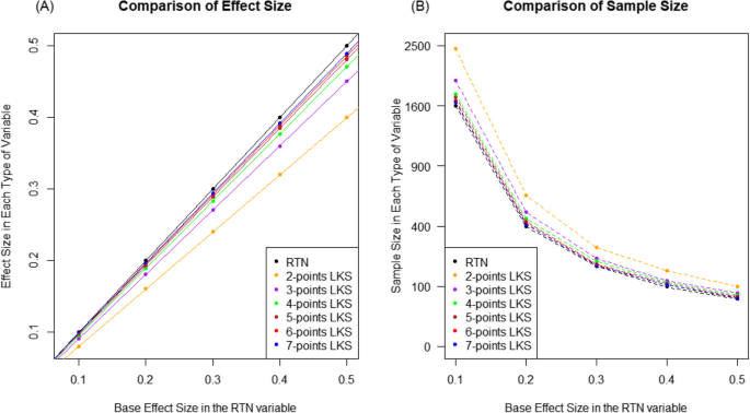
Effect size and required sample size according to the types of RTN and LKS variables. A Estimated effect sizes compared to that of the RTN variable. B Estimated required sample sizes to have 80% power for each effect size. Y-axis was drawn by square root transformed scale.
Afterward, we additionally examined the characteristics of the merged LKS variables and compared them with those of the merged RTN variables. Based on the settings explained in the method section, we calculated the statistical power and the required sample size for the LKS variable to match the statistical power of the RTN variable, and summarized the results in Table 2.
Table 2 Power analysis of two sample t-test with the multiple correlated RTN and LKS variables. Proportions (%) of significantly identified sets and their standard errors were provided. Required sample sizes were also presented in the parenthesis.
As shown in Table 2, the following trends were observed: First, when the number of merged variables was fixed, the pairwise correlation was inversely associated with the statistical power. Specifically, regardless of the variable type, the statistical power was highest at R = 0 and lowest at R = 1. These results were derived from the positive pairwise correlation, which increased the standard error of the mean difference, thereby decreasing the test statistic and increasing the p-value. Second, when the correlation between the variables was fixed, the statistical power increased as the number of merged variables increased, except when R = 1. This was because the number of pairwise correlations between the variables increased faster than the number of variances of the variables. For example, when there were two variables, both the number of pairwise correlations and the number of variances were two; however, these values were 90 and 10, respectively, when there were 10 variables. Therefore, the relative influence of the pairwise correlation on the standard error of the mean difference increases as the number of merged variables increases. Third, across all settings, the LKS variable with five or more points required an additional sample size of less than 10% compared to the sample size used in the RTN variables. This means that these types of variables had slightly lower but comparable efficiencies to obtain the same statistical power. Moreover, when the type of LKS variable was fixed, the required sample size was the largest at R = 0 or 1 and relatively small in the other correlation settings. This might be due to a decrease in the pairwise correlation during the conversion of the RTN variable into the LKS variable, which decreased the standard error and relatively improved statistical power compared to the results with R = 0 or 1.
Next, we additionally examined the extent to which the pairwise correlation was preserved during the transformation from the RTN to LKS variables. Specifically, we assessed preservation using the goodness-of-fit measures employed in the above two analysis methods [23]. Among the measures, we selected the GFI and SRMR [28], and Table 3 presents these two values for each LKS variable type. To align with the results in Table 2, we used the same settings for pairwise correlation (except R = 1) and number of variables.
Table 3 Goodness of fit measures (GFI/SRMR) between correlation matrices from the RTN and LKS variables. Their means and standard errors were provided.
In summary, the GFI value increased as the points of the LKS variable increased in all settings. However, in the R = 0 setting, the values did not exceed 0.95, which differed significantly from those in the other correlation settings. This is because the GFI calculated the relative improved similarity by comparing it with the identity correlation matrix and the RTN variables were also generated from the identity matrix. Consequently, the improved similarity was difficult to be high in this setting. However, in the other three correlation settings (R = 0.25, 0.5, and 0.75), all the GFI values significantly increased and exceeded 0.95, particularly in the LKS variable with four or more points. Subsequently, for SRMR, most values in the R = 0 setting were below 0.05. However, in the other three correlation settings, these values generally increased, staying below 0.05 only for the LKS variables with five or more points. Considering the results of these two measures, the LKS variables with five or more points exhibited desirable similarities to the RTN variables in terms of the correlation matrix during the transformation.
Finally, we examined the characteristics of the LKS variables when used as explanatory variables, as these variables may serve as predictors depending on their relationship with other variables in the study. After the analysis with the simulation settings explained in the method section was completed, we found several patterns in the results, as presented in Table 4. First, the statistical power increased as the number of explanatory variables increased in each combination of variable types. Second, the required sample size, to achieve the same statistical power as the results of the RTN explanatory variables, decreased as the number of explanatory variables increased. Third, as the number of points in the LKS variables increased, the required sample size decreased, reaching less than 220 for the five-point LKS variable. Combined with previous results, we concluded that the LKS variable with five or more points, not only as a response but also as an explanatory variable, may yield comparable results with those from the RTN variable.
Table 4 Power analysis of linear regression approach according to numbers of explanatory variables. Proportions (%) of significantly identified sets and their standard errors were provided. Required sample sizes were also presented in the parenthesis.