
This study uses results from an internally consistent, multi-model integrated framework developed by the Grid Operations Decarbonization Environmental and Energy Equity Platform (GODEEEP) project73 conducted at Pacific Northwest National Laboratory. The framework links a global human-Earth systems dynamics model with subnational detail in the US (Global Change Analysis Model-USA [GCAM-USA], an hourly electricity demand model (Total ELectricity Loads [TELL])74, a geospatial power plant siting model (Capacity Expansion Regional Feasibility [CERF])30,31, an hourly solar and wind generation model (Renewable Energy Potential [reV])75, and an hourly grid operations model (GridView)76. Model inputs are harmonized using a dynamically downscaled meteorological dataset following Representative Concentration Pathway 8.577, and downscaled US population78 projections following the Shared Socioeconomic Pathway 2 scenario. Through this multi-scale, dynamic process, we project high-resolution power plant deployment and grid operations in the Western US through 2050 in 5-year timesteps for two scenarios, high renewables and business-as-usual. Figure 6 presents the multi-model framework for the experiment for a single time-step. The sections below provide more details on each of the models in the integrated chain and the specifics of the power plant siting approach and land availability analysis.
Fig. 6: The Grid Operations Decarbonization Environmental and Energy Equity Platform (GODEEEP) multi-model framework.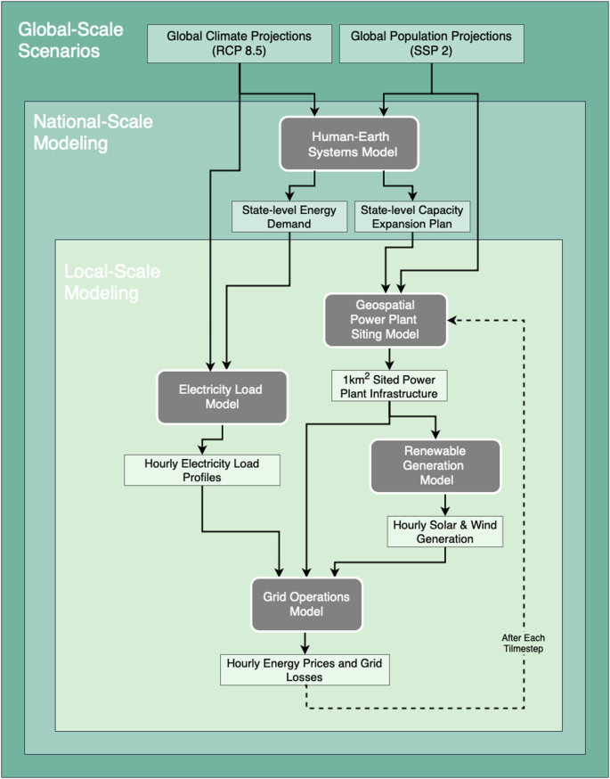
This framework demonstrates the connections (arrows) and data handoffs (white boxes) between models (dark gray boxes) in the multi-model experiment.
Global human-Earth system dynamics model with subnational detail for the US (GCAM-USA)
This study uses v6.0 of GCAM-USA, an open-source, dynamic recursive, human-Earth systems model that represents interactions across energy, agriculture, land, and water systems in 32 global regions, with subnational detail in the US, including all 50 states plus the District of Columbia79,80,81. GCAM-USA is a market equilibrium model that iteratively solves for a set of prices that simultaneously balances supply and demand across all markets in all regions in each modeling period (5-year time-steps). For example, model inputs for energy markets include supply curves to produce primary energy resources such as coal and natural gas, fixed and variable operating cost assumptions for electricity generation technologies (e.g., capital costs, heat rates, capacity factors), and price elasticities of demand. In the electricity market, technologies compete based on their levelized cost of energy (incorporates fixed and variable costs and assumed capacity factors). The levelized cost of energy is used in a logit formulation to address cost variability and prevent winner-takes-all outcomes in determining market shares. Based on the assumed capacity factors, GCAM-USA competes electricity generation technologies to serve different portions of a load duration curve with peak, sub-peak, intermediate, and baseload segments. For example, high capacity factor technologies such as coal and nuclear would compete to serve the baseload, while gas turbine-based technologies would compete to serve peak and sub-peak demands due to their lower capacity factors. The shape of the load duration curve is fixed in this version of GCAM-USA. It is scaled to represent the projected total electricity demand in each region at each time step.
In addition to supply curves, demand elasticities, and technology parameters, the model uses exogenous, region-specific, time series assumptions regarding population and economic growth, heating and cooling degree days, land availability, crop productivity, and runoff to calculate changing demands for energy, land, and water at each time step. The model can be forced with carbon dioxide emissions constraints or used with a reduced order climate model to target particular warming levels to represent alternative climate mitigation policies. Within the US, electricity generation, refined liquids production, and end use energy demands by buildings, transportation and industry are all modeled at the individual state level. Markets for oil, gas, and coal resolve nationally, and biomass feedstocks are modeled at a water basin scale (22 basins in the US). States are grouped to approximate the North American Electric Reliability Corporation grid regions and electricity trade is conducted across regions.
GCAM-USA simulates the high renewables and business-as-usual scenarios used in GODEEEP3 and passes its results to the other models in framework as shown in Fig. 6. The high renewables scenario includes emissions constraints to achieve a carbon-free US electricity system by 2035 and an economy-wide goal of net zero US greenhouse gas emissions by 2050. The business-as-usual scenario assumes a continuation of recent policies (as of 2024), including major state-level clean energy policies but does not include national net-zero economy goals. Both scenarios include US Inflation Reduction Act incentives for clean electricity generation, building energy efficiency, clean vehicle, and low-carbon fuels are in place between the years 2025 and 2035. Both scenarios also assume that carbon capture and sequestration technologies are available. The exogenous socioeconomic drivers are based on the Shared Socioeconomic Pathway 2, and heating and cooling degree days within the US include dynamic climate impacts using a projection based on the Representative Concentration Pathway 8.5 scenario.
As described in the following subsections, the other models in the framework use GCAM-USA’s state-level projections from each scenario for the annual demand for electricity, electricity generation by technology (including retirements), the national-scale projections of fuel prices, as well as GCAM-USA’s assumptions for electricity generation variable operating costs.
Power plant siting model (CERF)
CERF is a high-resolution, open-source power plant siting model30 that ingests regional capacity expansion plans and combines geospatial and economic analysis to determine feasible on-the-ground siting locations on a 1 km2 grid to evaluate the power plant landscape over time. CERF identifies sites for both renewable and non-renewable technologies using a suite of geospatial siting suitability data for dozens of specific power plant technology configurations (e.g., cooling types, turbine types, with or without carbon capture). By integrating the detailed geospatial suitability data31 with an economic algorithm, CERF selects optimal plant locations based on factors like grid interconnection costs and the locational marginal value of new generation (Fig. 7). These technology-specific sitings are provided on a 1 km2 basis in the form of x/y coordinates using the Albers Equal Area Conic projection. For this study, CERF evaluates the GCAM-USA electricity system expansion results for 11 states in the Western US: Arizona, California, Colorado, Idaho, Montana, Nevada, New Mexico, Oregon, Utah, Washington, and Wyoming.
Fig. 7: Capacity Expansion Regional Feasibility (CERF) model components.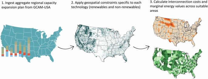
Step 1 shows a representation of coarse scale capacity expansion model output data. Step 2 shows an example geospatial siting exclusion layer for the contiguous US (excluded areas shown as dark green areas). Step 3 has a demonstration of distance (coloring) from transmission lines (solid black lines) across the contiguous US (top figure) and a demonstration of energy price zones (colors) and transmission lines (solid white lines) across the contiguous US.
CERF’s geospatial technology-specific suitability data determine the available installed capacity for each technology type that can be sited in a 1 km2 area. For non-renewables, this corresponds with the total project capacity (e.g., natural gas combined cycle capacity of 727 MW6). For wind and solar PV this corresponds with the rated capacity of the wind turbines and the solar arrays that can be placed within a 1 km2 area. For solar, we conducted an analysis of the spatial footprints of existing single-axis utility scale solar projects in Western US states82 and evaluated the total rated direct current (DC) capacity per project area assuming 75% of project land area is allocated to solar arrays directly10. This analysis showed that the majority of values fell in the range of 20–60 MWDC/km2. A value of 30 MWDC/km2 was chosen for CERF single-axis PV model runs as it aligned with assumptions provided in the literature which estimated capacity density of solar PV based on a best-fit analysis of values found in the previous studies which gave a value of 30.0583. Recent studies have shown that rated capacity densities of new installations of solar may be in the higher portion of this range68 and that previous literature may be underestimating the available capacity. Higher capacity densities for solar PV would decrease the total amount of land required. However, recent increases in setback requirements may limit improvements in this space18. To account for this uncertainty, the exploratory sensitivity analysis presented in Section “Sensitivity analysis of increasingly restrictive siting policies identifies cases where projected generation needs cannot be met, implying the need for policy coordination” evaluates single-axis solar PV capacity densities between 15–60 MWDC per km2 to evaluate projected future generation under a range of rated capacity scenarios. We additionally discuss the implications of lower capacity density assumptions for solar PV in the “Limitations” section.
Rated wind capacity per km2 can vary considerably by project due to differences in required turbine spacing, turbine characteristics, setbacks, and a multitude of other factors. Recent estimates of individual rated wind turbine capacity place the value at approximately 3 MW6 per turbine and projections of average rated capacities in 2035 are 5.5 MW per turbine84. Due to the computational complexity of the integrated experiment, a simplified approach is used to allocate rated wind capacity to km2 for CERF model runs. In our experiment we assume approximately three wind turbines per km2 based on an assumed rotor diameter of 130 m6 and spacing of 3–4 rotor diameters apart while noting that these are typically highly site- and technology-specific components. While this method does not capture site-level variation, it offers a tractable approximation for large-scale integrated experiments where more detailed modeling is infeasible. Future research in this space aims to enhance this modeling to capture local factors that influence turbine spacing and wind farm layout. The spacing between turbines is heavily dependent on primary wind direction which is not currently considered in the modeling and remains an area for future development. Under multi-directional wind conditions or when turbines have longer rotor diameters, for example, the required spacing between turbines can be much higher, leading to lower capacity density assumptions85. The total available rated wind capacity assumed in the CERF model is the sum of the assumed rated capacity across turbines in each km2, which is assumed to increase over time. For 2025 and 2030 runs capacity density corresponds to 12 MW/km2, for 2035 and 2040, this corresponds to 16 MW/km2, and for 2045 and 2050 runs this corresponds to 21 MW/km2, representing large technological advancements and land use efficiency improvements over time, aligning with recent trends in wind technology scaling84,86. These values are higher than historic estimates found in the literature9, which gives an average of just over 5 MW/km2, however, these estimates are only for plants operational prior to 2009 and rated turbine capacities have since increased86. Other literature suggests that most capacity density per km2 estimates for wind overestimate land allocated to spacing areas and include spacing areas between turbine clusters and areas on wind farm edges87. These researchers found that removing these areas led to a mean installed power density of nearly 20 MW/km2 for existing international installations as of 2021. The methodology used within this study makes it more challenging to compare to empirically-based estimates, however68. Substantial variation exists in the literature on estimating values for existing facilities. Recent estimates68 using harmonized methodologies, which were published after the completion of this analysis, have shown that values of existing sites may be even lower than 5 MW/km2 which could have large implications for future land use if future values are aligned closer to these estimates. We discuss this recent research and what it could mean for future land use projections in the “Limitations” section. To capture uncertainty related to rated capacity per km2 for wind, the exploratory sensitivity analysis presented in Section “Sensitivity analysis of increasingly restrictive siting policies identifies cases where projected generation needs cannot be met, implying the need for policy coordination” evaluates wind capacity densities in 2050 between 6–24 MW/km2 and evaluates generation at both 100 m and 120 m hub heights. There is considerable uncertainty surrounding technology advancement in future years, future work in this area aims to explore this uncertainty in the experiment modeling structure directly.
The economic algorithm in CERF determines individual power plant locations through a competitive process, considering technology-specific costs for connecting to the nearest substation and natural gas pipeline (if necessary), along with the technology-specific value of new generation in that location based on wholesale electricity prices (locational marginal prices) from GridView. Specific generation technology costs and parameters including heat rate, variable operations & maintenance, fuel cost, and technology operating life are also gathered from GCAM-USA for each timestep and factor in to the economic algorithm to determine operating cost in each location on an annualized basis30. Considering dynamic factors such as protected lands, population density, existing infrastructure, and water availability, CERF serves as a form of ground-truthing to both ensure the viability of broader expansion planning models and depict the evolution of the power plant landscape under various climate, socioeconomic, technological, and policy scenarios. Population-density based siting restrictions used in CERF are consistent with Shared Socioeconomic Pathway 2 population projections in each run year78.
reV renewable generation model
reV is an open-source renewable generation model that assesses resource potential given specific wind and solar farm characteristics75. In each run year, solar and wind farm configuration and location data is collected from CERF and run through reV to provide hourly resource profiles. The wind and solar models require several meteorological inputs. The wind model requires pressure, temperature, wind speed, and wind direction at the turbine hub height. The solar model requires temperature, pressure, wind speed and solar irradiance. The solar irradiance must be supplied in the form of global horizontal, diffuse normal, and diffuse horizontal irradiance. A complete description of the wind and solar data preprocessing and their evaluation is described in Campbell et al.88. Climate data used in reV to create the generation output is consistent with the Representative Concentration Pathway 8.5 (hotter) climate scenario used throughout the GODEEEP experiment77.
TELL hourly electricity load model
The TELL model74 projects hourly electricity demand over time in response to weather and climate variability. The model is machine learning-based and was trained on historical hourly meteorology and energy demand data for 54 balancing authorities in the US. TELL takes as input the annual state-level total electricity demand projections from GCAM-USA and downscales them to hourly load time-series at the county-, state-, and BA-scale. Loads across all scales coming out of TELL are conceptually and quantitatively consistent. The electricity demand projection used in the GODEEEP experiment are publicly available89.
GridView
GridView76 is a proprietary grid operations tool that models transmission and optimization of electric grid resources. Power plant locations and their grid interconnection points provided by CERF30, as well as renewable generation profiles from reV75, are imported into GridView, which solves a Unit Commitment and Economic Dispatch optimization problem to determine the least-cost dispatch solution that meets electricity demand, reserve requirements, and other operating constraints. Operational costs and parameters for each technology type such as fuel cost, variable operations & maintenance, and heat rate are provided to GridView from GCAM-USA in each timestep to maintain consistency regarding operational assumptions. Hourly electricity demands are provided by TELL74. At each hour of the year, GridView minimizes the total system operating cost by selecting the most economical combination of generation units and transmission capacities, while satisfying a range of constraints. These include unit-specific constraints (e.g., generator capacity limits, minimum operating times, ramp rates) and system-wide constraints (e.g., transmission capacity limits, operating reserves, and emission constraints). The optimization algorithm (FICO XPRESS) used to solve the Unit Commitment/Economic Dispatch problem, formulated as a Mixed Integer Linear Programming Problem (MILP), ensures that the solution is feasible in the sense that all constraints are met without violating any limits. If any incompatibility between the newly added generation and GridView’s constraints is detected (e.g., excessive generation that cannot be effectively used in the dispatch or inefficient generation to meet demand), GridView addresses the issue by shedding load or generation through appropriately designed penalties and dispatch costs. This adjustment guarantees optimality in the sense that the load balance constraint is satisfied at each simulated hour, meaning that the total generation matches the total demand (plus reserves) for each time step, and the system operates efficiently under the given constraints.
The integrated engineering and economic analysis conducted by the model produces locational marginal prices for each substation in its nodal network. These locational marginal prices are used by the CERF model in subsequent timesteps to determine net operating value from each interconnection point on the grid. Note that the substation infrastructure network is assumed to remain consistent throughout the experiment timeline. GridView was chosen as the appropriate grid operations model for the GODEEEP experiment because it is a commonly used tool by long-term and operational planners in utilities across the Western US.
Determining the land usage of power plant additions and retirements
Land usage in this analysis corresponds with project-level land use of the generation facility. Each km2 accounts for the generation infrastructure, spacing between wind turbines, spacing between solar arrays, buildings, and other supplemental infrastructure necessary for plant operation. Indirect land usage beyond the direct generation facility is not included in the total land usage. Examples of indirect land usage not covered here can include cropland for corn based ethanol production for biomass90 and mining facilities for coal, natural gas, and petroleum production91.
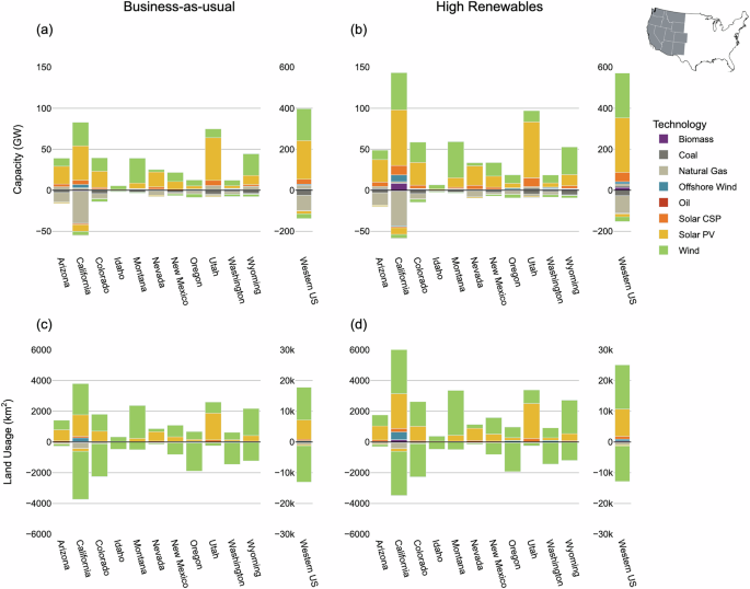
Direct converted land estimates are discussed in Section “30% more land dedicated to solar and wind generation is needed in the Western US under a high renewables scenario compared to a business-as-usual scenario” and provided in Supplementary Table 6 by state and technology. For wind, we analyze a range of 2–5% of project area that corresponds with directly converted land37. For solar PV, direct land use can vary considerably and was approximated based on the ratio of total land use per MW and direct land use per MW for various utility scale systems10. To capture a range of values, we analyzed direct land use for 60, 75, and 90% of project area. For all other technologies, the converted land fraction is assumed to be close to 100% of project area with minimal land available for alternative applications. The range applied to these technologies, therefore, is 90, 95, and 100%.
To calculate the land usage of pre-existing power plants that are retired in the experiment timeframe (Fig. 1) on an equivalent basis as new additions which are sited by the CERF model, point geometry locations of non-CERF-sited generation facilities were converted to 1 km2 polygon geometries by square buffering point locations by 500 m. For utility-scale non-renewable facilities, this aligned with the 1 km2 land usage assumption in CERF directly. For renewable facilities, point location data for existing individual wind turbines and solar array locations were also buffered by 500 m and then spatially joined to capture overlap as interior project space. To determine the amount of previously occupied land that became free for other non-generation purposes after facility retirement, any land occupied by new siting additions was spatially subtracted from land that saw retirement. This effectively removes land from the total that had facility retirement but then saw new generation overtake the space. This method was chosen to best represent the amount of land dedicated to electricity generation by 2050 in Fig. 1 under each scenario.
Evaluation of power plant siting interactions with DACs, important farmland, and natural areas
To gain insight into the amount of projected power plant sitings and associated land usage that intersects with areas of interest, we use high resolution geospatial raster data layers. These areas include federally identified DACs, combined important farmland, and composite natural areas. This section describes the methodology behind the projected infrastructure siting intersection analysis. Documented code to reproduce this analysis is provided in this article’s meta-repository92 (see “Code availability” section).
First, we use CERF power plant siting projections for both the high renewables and business-as-usual scenarios from the experiment workflow shown in Fig. 6 to determine the coordinates of new infrastructure sitings. Second, we overlay vector point CERF sitings on 1 km2 resolution geospatial raster representations of our areas of interest. Last, we use geospatial analysis to sum the number of intersections between power plant points and grid cell representations of indicated areas to determine the total number of km2 of sitings by technology.
Spatial representations of DACs, natural areas, and important farmland were collected from the Geospatial Raster Input Data for Capacity Expansion Regional Feasibility (GRIDCERF) database31,32 which provides a binary representation of the contiguous US that meet or do meet a specific criterion at a 1 km2 resolution.
Federally identified DACs include any census tract that is designated by the US Center for Environmental Quality as disadvantaged due to water, energy, climate, workforce, pollution, health, or transportation reasons as of 202453. Federally-identified DACs were included as an exclusion in our sensitivity analysis to capture a scenario in which these communities reject development of new power plant infrastructure due to potential adverse impacts40,47,48,49.
Important farmland includes any area designated by the U.S. Department of Agriculture as prime farmland, farmland of state importance, farmland of local importance, or farmland of unique importance54. These areas have higher soil quality and moisture supply, indicating that they are valuable for agricultural purposes. We investigate the potential impacts if these lands were excluded from new power plant siting.
Natural areas are comprised of 28 unique environmental areas from the GRIDCERF database associated with undisturbed natural areas, protected natural areas, viewsheds, protected habitats, and similar. These layers can include areas such as US National Parks, national marine sanctuaries, scenic and recreational areas, US Bureau of Land Management outstanding natural areas, wilderness areas, wild and scenic rivers, and many others. For the full list of layers included in the compiled natural area designation, refer to Supplementary Table 5.
Evaluating 2050 high renewables scenario solar PV and wind generation feasibility under various siting constraint combinations
We analyzed 27 different land suitability scenarios (Table 1) as part of our analysis to determine the feasibility of a high renewables capacity expansion plan under additional power plant siting restrictions. We began with the baseline siting exclusions for each technology (see Supplementary Tables 1 and 2) and layered additional exclusions including DAC areas, important farmland, three different levels of environment protection (Level 1, Level 2, and Level 3), three different levels of spatial buffer around environmental areas (1 km, 5 km, and 10 km), and various combinations of each.
New geospatial raster layers were created for each of the siting suitability constraint scenarios where additional restrictions were layered onto existing siting restrictions for the given technology. For example, under the DAC scenario, the composite raster layer excludes all areas from siting that are either (1) included in baseline siting exclusion areas or (2) in a federally identified DAC. The baseline siting considerations for this analysis are consistent with Shared Socioeconomic Pathway 2 populations for 2050, to capture downscaled population dynamics within the 2050 GCAM-USA simulations. Baseline siting layers for solar and wind represent technology and policy siting constraints as of 202432.
Varying the degree of environmental area exclusion (Levels 1–3) is intended to determine the degree of generation potential if new areas are excluded from development above and beyond what is excluded from siting as of 2024. These include applying any current natural area exclusions that apply to either solar or wind to both solar and wind (Level 1), adding additional areas of high environmental risk (e.g., golden eagle habitats) (Level 2), and adding areas of moderate risk (e.g., golden eagle distribution) and above (Level 3). The designation of high risk and moderate risk areas is leveraged directly from U.S. Bureau of Land Management’s wind development assessment of the Western US93. Though some of the restrictions in Level 1 only apply to solar or wind, we decided to include Level 1 as an analysis to capture examples of new restrictions that exclude entire subregions from any renewable development26, regardless of whether one technology may be less impactful than another. Information with each of the individual areas included in Level 1, Level 2, and Level 3 is provided in Supplementary Table 5.
In addition to varying the level of natural area protection, we also tested how sensitive results are to increasing the spatial area of existing and new environmental exclusion areas. The intention of this analysis is to determine if new policies that place additional buffers on environmental areas are particularly impactful to generation goals. One kilometer, 5 km, and 10 km were chosen as buffers to represent small, intermediate, and large buffered areas. Though there are examples of new policies that stretch beyond 10 km22, our results indicate that buffers beyond 10 km yield similar outcomes given the quantity of natural areas in the Western US.
To determine the resource potential within the remaining land area after each exclusion, we used 2050 capacity factor projections for solar and wind coincident with an Representative Concentration Pathway 8.5 (hotter) scenario94. The dataset employs regional atmospheric climate model results to produce wind and solar power generation throughout the contiguous US at a 1/8th degree (12 km2) resolution which was downscaled to 1 km2 for this analysis. For wind, these capacity factors are provided at the 125-meter height to be as consistent as possible with our 120-meter turbine hub height assumption used in the analysis. Total annual generation (in megawatt-hours), for each region subject to siting restrictions is determined by summing the product of the assumed rated technology power capacity in MW and the sum of hourly capacity factors in each grid cell across all hours of the year, across all available grid cells within the region.
Total area includes land used directly by each technology as well as land for clearance, buildings, roads, and other areas included in the site boundary. The sensitivity analysis was conducted under four capacity density assumptions for wind (6, 12, 18, and 24 MW/km2) and single-axis solar PV (15, 30, 45, and 60 MW/km2) as well as two wind turbine hub height (100 m and 120 m) assumptions. The sensitivity analysis results can be found in the Supplemental Information and in the paper’s meta-repository92.
Total generation potential was aggregated to various spatial boundaries including GCAM-USA trading region level, each of the 11 Western US states individually, and the Western US region as a whole (sum of all 11 states). Note that GCAM-USA electricity trading regions are approximated to state boundaries. There are three electricity trading regions in the Western Interconnection according to GCAM-USA: the Northwest Grid (Oregon, Washington, Idaho, Montana, Nevada, Utah), the Southwest Grid (Arizona, New Mexico, Colorado, and Wyoming), and the California Grid (California). GCAM-USA trading regions are defined within the GCAM-USA model as clusters of states that have the capability to trade energy amongst one another and follow the US Department of Energy’s Energy Information Administration National Energy Modeling System Electricity Market Module Regions95.
The target solar and wind generation for 2050 under the high renewables scenario in each trading region is determined by summing generation across all states within each trading region in the GODEEEP GCAM-USA simulation output3. Total generation potential for solar and wind under each siting suitability scenario were compared to the target generation level to determine the ability to meet generation requirements. Scenarios in which available generation in a specified area was less than target generation for the same specified area was an indication that the remaining available land did not contain adequate resource potential to provide the total target generation.