
Variable-trajectory
Let \(y_{it} \in {\mathbb{R}}\) denote the observed response value for the subject \(i \in \left\{ {1, \ldots ,n} \right\}\) at the time point \(t \in \left\{ {1,…,T_{i} } \right\}\), where \(T_{i}\) is the number of observations for subject i. The response trajectory for subject i can be represented as the vector.\(Y_{i} = (y_{i1} ,y_{i2} , \ldots ,y_{{iT_{i} }} )^{{\text{T}}} .\)
The collection of these trajectories for all subjects can be organized in a response matrix.
\(Y = [Y_{1} ,Y_{2} ,…,Y_{n} ]^{{\text{T}}}\), with each row corresponding to a subject’s longitudinal response profile.
$$ Y = \left( \begin{gathered} Y_{1} \hfill \\ Y_{2} \hfill \\ \vdots \hfill \\ Y_{n} \hfill \\ \end{gathered} \right) = \left[ {\begin{array}{*{20}c} \begin{gathered} y_{11} \hfill \\ y_{21} \hfill \\ \end{gathered} & \begin{gathered} \ldots \hfill \\ \ldots \hfill \\ \end{gathered} & \begin{gathered} y_{{1T_{1} }} \hfill \\ y_{{2T_{2} }} \hfill \\ \end{gathered} \\ \vdots & \ddots & \vdots \\ {y_{n1} } & \cdots & {y_{{nT_{n} }} } \\ \end{array} } \right] $$
(1)
Distances in the D quantitative covariates and the T measurement times
Let \(X_{it}\) denote the covariate vector for subject i at time t, and \(X_{it}^{\left( k \right)}\) denote the k-th as the covariate component. We use \(X_{i.}\) to represent the longitudinal covariate matrix for subject i and \(X_{..}\) to denote the full covariate matrix for all subjects across all time points.
Therefore \(X_{it} = (X_{it}^{\left( 1 \right)} ,{\text{ X}}_{it}^{\left( 2 \right)} , \, \ldots ,{\text{ X}}_{it}^{\left( D \right)} ) \in {\mathbb{R}}^{D}\), denote the D-dimensional covariate vector for subject i at time point t. To quantify the similarity between two such observations, a distance metric can be used. A common choice is the Euclidean distance, defined as follows:
$$ d_{t} (X_{it} ,X_{jt} ) = \sqrt {\sum\limits_{k = 1}^{D} {\left( {X_{it}^{(k)} – X_{jt}^{(k)} } \right)^{2} } } $$
(2)
Or Mahalanobis distance accounting for correlation in predictors:
$$ d\left( {X_{it} ,X_{jt} } \right) = \sqrt {(X_{it} – X_{jt} )^{T} \Sigma^{ – 1} (X_{it} – X_{jt} )} $$
(3)
where Σ is the covariance matrix of covariance matrix of the D-dimensional covariates across subjects.
Let \( X_{i..} ,X_{j..} \in {\mathbb{R}}^{T \times D}\) denote the longitudinal covariate matrices for subjects i and j, respectively. Then, it \(d(X_{i..} ,X_{j..} )\) represents the distance between these two matrices, computed based on a suitable aggregation of temporal or feature-wise distances. Two methods were used to determine this distance between two matrices. The two matrices’ T columns are considered first, followed by the calculation of distances between the T couples of columns, and, lastly, the combination of these T distances using a function combining the column distances. The second method involves considering the D lines of the two matrices, calculating the distances between the D line pairs, and then using a function that combines the line distances, to sum up these D distances.
More formally, to compute a distance between \(X_{i..}\) and \(X_{j..}\) according to the first method, for each fixed time point t, let \(X_{it} ,X_{jt} \in {\mathbb{R}}^{D}\) denote the covariate vectors for subjects i and j, respectively, at time t. The distance between these vectors is defined as:
$$ d_{t} (X_{it} ,X_{jt} ) = \sqrt {\sum\limits_{k = 1}^{D} {\left( {X_{it}^{(k)} – X_{jt}^{(k)} } \right)^{2} } } $$
(4)
This corresponds to the Euclidean distance between the covariate vectors at time t for subjects i and j, extracted from their respective longitudinal matrices \(X_{i.}\) and \(X_{j.}\). The result is a vector of T distances \(\left( {d_{1} \left( {X_{i1} ,X_{j1} } \right),d_{2} \left( {X_{i2} ,X_{j2} } \right), \ldots ,d_{T} \left( {X_{iT} ,X_{jT} } \right)} \right)\). Then, these T distances can be combined using a function that algebraically corresponds to a norm \(\left\| \cdot \right\|\) of the distance vector. Finally, the distance between \(X_{i.}\) and \(X_{j..}\)
$$ d\left( {X_{i..} ,X_{j..} } \right) = \left\| {d_{1} \left( {X_{i1} ,X_{j1} } \right),d_{2} \left( {X_{i2} ,X_{j2} } \right), \ldots ,d_{T} \left( {X_{iT} ,X_{2T} } \right)} \right\| $$
(5)
To compute the distance \(d^{\prime}\) between the longitudinal data matrices \(X_{i..}\) \(X_{j..}\) according to the second approach, we define the distance \(d_{k} \left( {X_{i.}^{\left( k \right)} ,{\text{ X}}_{j.}^{\left( k \right)} } \right)\) between the time series of the k-th variable for both subjects. Here, they \(X_{i.}^{\left( k \right)} ,X_{j.}^{\left( k \right)} \in {\mathbb{R}}^{T}\) represent the temporal trajectories of covariate k for subjects i and j, respectively. The overall distance is then computed by aggregating over all variables:
$$ d^{\prime}(X_{i..} ,X_{j..} ) = \sum\limits_{k = 1}^{D} d (X_{i.}^{\left( k \right)} ,X_{j.}^{\left( k \right)} ) $$
(6)
This results in a vector of D distances. \(d_{1} \left( {X_{i.}^{\left( 1 \right)} ,X_{j.}^{\left( 1 \right)} } \right),d_{2} \left( {X_{i.}^{\left( 2 \right)} ,X_{j.}^{\left( 2 \right)} } \right), \ldots ,d_{D} \left( {X_{i.}^{\left( D \right)} ,X_{j.}^{\left( D \right)} } \right)\).
Then, we combine these D distances using a function that algebraically corresponds to a norm \(\left\| \cdot \right\|\) of the distance vector. Finally,
$$ d^{\prime}(X_{i..} ,X_{j..} ) = \left\| {d_{1} \left( {X_{i.}^{\left( 1 \right)} ,X_{j.}^{\left( 1 \right)} } \right),d_{2} \left( {X_{i.}^{\left( 2 \right)} ,X_{j.}^{\left( 2 \right)} } \right), \ldots ,d_{D} \left( {X_{i.}^{\left( D \right)} ,X_{j.}^{\left( D \right)} } \right)} \right\| $$
(7)
The choice of the norm \(\left\| \cdot \right\|\) can lead to the definition of many distances. On the contrary, in the case where \(\left\| \cdot \right\|\) the standard p-norm is the Minkowski distance with parameter p, choosing either method \(d\) \(d^{\prime}\) leads to the same result:
$$ d(X_{i..} ,X_{j..} ) = d^{\prime}(X_{i..} ,X_{j..} ) $$
The proof is based on [20]:
$$ d(X_{i..} ,X_{j..} ) = \sqrt[p]{{\sum\limits_{t} {\left( {d\left( {X_{it} ,X_{jt} } \right)} \right)^{p} } }} = \sqrt[p]{{\sum\limits_{t} {\left( {\sqrt[p]{{\sum\limits_{k} {\left( {\left| {X_{it}^{\left( K \right)} – X_{jt}^{\left( k \right)} } \right|^{p} } \right)^{p} } }}} \right)^{p} } }} $$
$$ \sqrt[p]{{\sum\limits_{t} {\sum\limits_{k} {\left| {X_{it}^{\left( k \right)} – X_{jt}^{\left( k \right)} } \right|^{P} = \sqrt[p]{{\sum\limits_{t} {\left( {\sqrt[P]{{\sum\limits_{K} {\left( {\left| {X_{it}^{\left( k \right)} – X_{jt}^{\left( k \right)} } \right|^{P} } \right)} }}} \right)} }}} } }} $$
$$ = \sqrt[p]{{\sum\limits_{k} {\left( {d\left( {X_{i.}^{\left( k \right)} – X_{j.}^{\left( k \right)} } \right)} \right)^{p} } }} = d^{\prime}\left( {X_{i..} ,X_{j..} } \right) $$
(8)
Therefore, the Minkowski distance, a generalization of the Euclidean distance, is used in this study as the basis for computing similarity between multivariate profiles [20].
$$ d\left( {X_{i..} ,X_{j..} } \right) = \sqrt[p]{{\sum\limits_{t,k} {\left| {X_{it}^{\left( k \right)} – X_{jt}^{\left( k \right)} } \right|^{p} } }} $$
(9)
The Euclidean distance is obtained by setting p = 2, the Manhattan distance by setting p = 1, and the maximum distance by passing to the limit \(p \to + \infty\)[20].
K-Nearest Neighbors (KNN) regression
KNN is a non-parametric method for regression and classification, which is part of the non-parametric approach of local averaging. In this non-parametric approach, the estimation \(m(x_{i} ) = E(Y_{i} \left| {x_{i} )} \right.\) is obtained by averaging the values of data points \(y_{j}\) whose corresponding \(x_{j}\) predictors are close to \(x_{i}\) the target point. It means that
$$ \hat{m}\left( {x_{i} } \right) = \sum\limits_{j = 1}^{n} {w_{j} } \left( {x_{i} ;x_{1} ,…,x_{n} } \right)y_{j} = \left( {w_{1} (X),w_{2} (X),…,w_{n} (X)} \right)\left( \begin{gathered} y_{1} \hfill \\ y_{2} \hfill \\ \vdots \hfill \\ y_{n} \hfill \\ \end{gathered} \right) $$
(10)
where the weights \(w_{j} \left( {x_{i} ;x_{1} ,…,x_{n} } \right)\) are non-negative and decrease as the distance between \(x_{j} ;j = 1,…,n\) and \(x_{i}\) increases. This approach helps estimate the value \(y_{i}\) corresponding to \(x_{i}\) a target point by borrowing information from nearby observations. It assigns greater weight to observations closer to the target point \(x_{i}\) and less weight to those farther away [22].
KNN regression for longitudinal data
In longitudinal studies, Y values for each individual consist of multiple measurements taken over time. However, the main problem of examining the effect of independent variables on the response remains. As stated in Eq. (1), \(Y\) is a matrix containing a quantitative variable trajectory whose i-th row represents the trajectory response variable for the i-th individual to estimate the variable-trajectory vector of a new individual using KNN regression; we denote this by \(\hat{y}_{it}\). In this case, the nearest neighbors of covariate trajectory \(X_{i.}\) are using the distance metric in Eq. (9). The predicted response trajectory is computed as the weighted average of the neighbors’ outcomes [23]. To predict the value of the response variable for subject i at time t, we use the average response of its k-nearest neighbors, identified based on longitudinal distances between their covariate trajectories \(X_{i.}\):
$$ \hat{y}_{it} = \sum\limits_{{j \in N_{k} \left( i \right)}} {\frac{1}{k}y_{jt} } $$
(11)
where \(\hat{y}_{it}\) denotes the predicted response for subject i at time t, obtained via local averaging over the responses of the k-nearest neighbors. The prediction is computed as the average of the outcomes of the nearest neighbors at time t.
Where N(i) denotes the set of indices corresponding to the k-nearest neighbors of subject i, based on the longitudinal distance between their covariate trajectories.
Alternatively, it can be used as weighted averaging:
$$ \overset{\lower0.5em\hbox{$\smash{\scriptscriptstyle\frown}$}}{m} (X_{it} ) = \sum\limits_{{j \in N_{k} \left( i \right)}} {w_{j} \underline {y}_{jt} } $$
$$ with \, weights\;\;w_{j} = \frac{{1/d\left( {X_{i \cdot } ,X_{j \cdot } } \right)}}{{\sum\limits_{l\smallint N\left( i \right)} 1 /d\left( {X_{i \cdot } ,X_{l \cdot } } \right)}} $$
(12)
where \(d(X_{it} ,X_{jt} )\) denotes the longitudinal distance between subjects i and j at time t, and weights are normalized inverse distances to emphasize closer neighbors. The above method requires that the covariates \(X_{i.}\) be time-dependent and can sufficiently explain Y. We will refer to this method as KNNRLD (KNN Regression for Longitudinal Data).
Some drawbacks related to KNN regression
Although KNN has proved to be a ubiquitous classification or regression tool with good scalability, it has some drawbacks. One of its most significant drawbacks is that it is a lazy learner, i.e., it uses all the training data at runtime [2]. Another issue is that KNN regression is prone to the curse of dimensionality. KNN estimators are universally consistent, which means.
$$ {\rm E}(\hat{m}_{k} – m)^{2} \to 0\;as\;n \to \infty $$
(13)
However, KNN regression estimators may perform poorly if the input space dimension is high (i.e., the number of covariates, p). This is simply because the nearest neighbors must be close to the target point, which can lead to significant errors in high-dimensional spaces. So, it can be proved that
$$ {\rm E}(\hat{m}_{k} \left( x \right) – m\left( x \right))^{2} \le n^{{ – \frac{2}{2 + P}}} $$
(14)
This is a relatively weak error rate because it depends weakly on the dimension p. Therefore if we want the maximum estimation error to be less than or equal to \(\varepsilon \ge 0\) that is
$$ {\rm E}(\hat{m}_{k} \left( x \right) – m\left( x \right))^{2} \le \varepsilon $$
(15)
Therefore, the number of samples n should be chosen so that
$$ n \ge \varepsilon^{{ – \frac{2}{2 + P}}} $$
(16)
Which increases exponentially with the increase of P [24].
To generalize KNN regression in longitudinal data, first consider the assumption that none of the independent variables change over time, so the sample size can be established based on Eq. (11) for KNN regression in longitudinal data because, in this case, the original k-nearest neighbor is the same as a P-dimensional KNN regression for cross-sectional data. However, we will assume that all the independent variables used in KNN regression with longitudinal data are time-dependent. In this case, we first return to Eq. (8), where
$$ \sqrt[p]{{\sum\limits_{t} {\left( {d\left( {X_{it} ,X_{jt} } \right)} \right)^{p} } }} = \sqrt[p]{{\sum\limits_{t} {\left( {\sqrt[p]{{\sum\limits_{k} {\left( {\left| {X_{it}^{\left( k \right)} – X_{jt}^{\left( k \right)} } \right|^{p} } \right)^{p} } }}} \right)^{p} } }} $$
(17)
That is, the problem of the distance coefficient between subjects i and j can be separated into the problem of finding the distance coefficient in the shortest possible time. Therefore, \(t = 1,2, \ldots ,T\) the required sample volume will be obtained at any measurement time, similar to the previous state. The required sample size for the case where some independent variables depend on time is between these two cases.
As mentioned, the curse of dimensionality in a KNN estimator is that the nearest neighbors must be close to the target point. High dimensionality can lead to significant errors. This problem can be partially mitigated by clustering the data before running the K-Nearest Neighbors (KNN) algorithm. Clustering helps by grouping similar subjects, thereby confining the nearest-neighbor search to localized regions in the feature space. As a result, the influence of high dimensionality is reduced because distance computations are performed within smaller, denser subsets rather than across the entire space. This strategy is particularly effective for longitudinal data, where local structures often carry more meaningful temporal relationships. By clustering subjects based on proximity in the P-dimensional space, the KNN algorithm operates within more homogeneous groups. Additionally, distance calculations are performed on smaller subsets of data (as opposed to full n-dimensional matrices), which improves computational efficiency—especially for large-scale longitudinal datasets [20, 25].
Enhancing KNN regression accuracy through clustering in longitudinal data
By clustering individuals based on similar temporal patterns and covariate structures, the overall variability within each group is reduced. This approach ensures that subjects with comparable characteristics are analyzed together, leading to a more consistent intra-cluster correlation. As a result, applying KNN regression within each cluster becomes more stable and reliable. Rather than implementing KNN across the entire dataset, restricting it to pre-defined clusters allows the algorithm to find neighbors with more similar longitudinal structures. This localized approach improves predictive accuracy by ensuring comparisons among more relevant observations. When individuals within a cluster exhibit shared underlying characteristics, such as similar baseline values or progression trends—clustering effectively accounts for these latent factors. It reduces the necessity for explicitly modeling random effects, simplifying the regression process while capturing subject-specific influences [12, 21, 25].
The objective of CKNNRLD is to estimate the value of a longitudinal outcome, yit, using observed covariates, Xit, through a cluster-based nearest-neighbor regression framework. This framework aggregates information from similar time-aligned individuals to produce continuous-valued predictions.
Clustering-based KNN regression for longitudinal data
The algorithm comprises both preprocessing and processing steps, as outlined below.
Preprocessing steps
1.
Clustering variable trajectories with the help of K-means for longitudinal data (KML) method [19, 20]
2.
Finding the optimal number of clusters using the Calinski criterion [26] or the other criteria in the kml package [19, 20] (in this step, users can determine the number of clusters according to their taste based on prior information about the data).
3.
Determining the optimal K for KNN regression by k-fold cross-validation method (If the clusters are homogeneous, one same K can be used for all the clusters.)
4.
Finding the representative of each cluster (the mean vector (matrix for time-dependent data) of the corresponding covariate variables in each cluster).
5.
Saving the information from the previous four steps.
Processing steps
6.
Finding the cluster where the query point (query vector for non-time-dependent data and query matrix for time-dependent data) has the highest probability of occurrence (the smallest distance to the representative of each cluster).
7.
KNNRLD is applied based on the weighted average of K nearest neighbors of query variables in the desired cluster.
8.
The value calculated in the previous step is a new variable trajectory provided as an output.
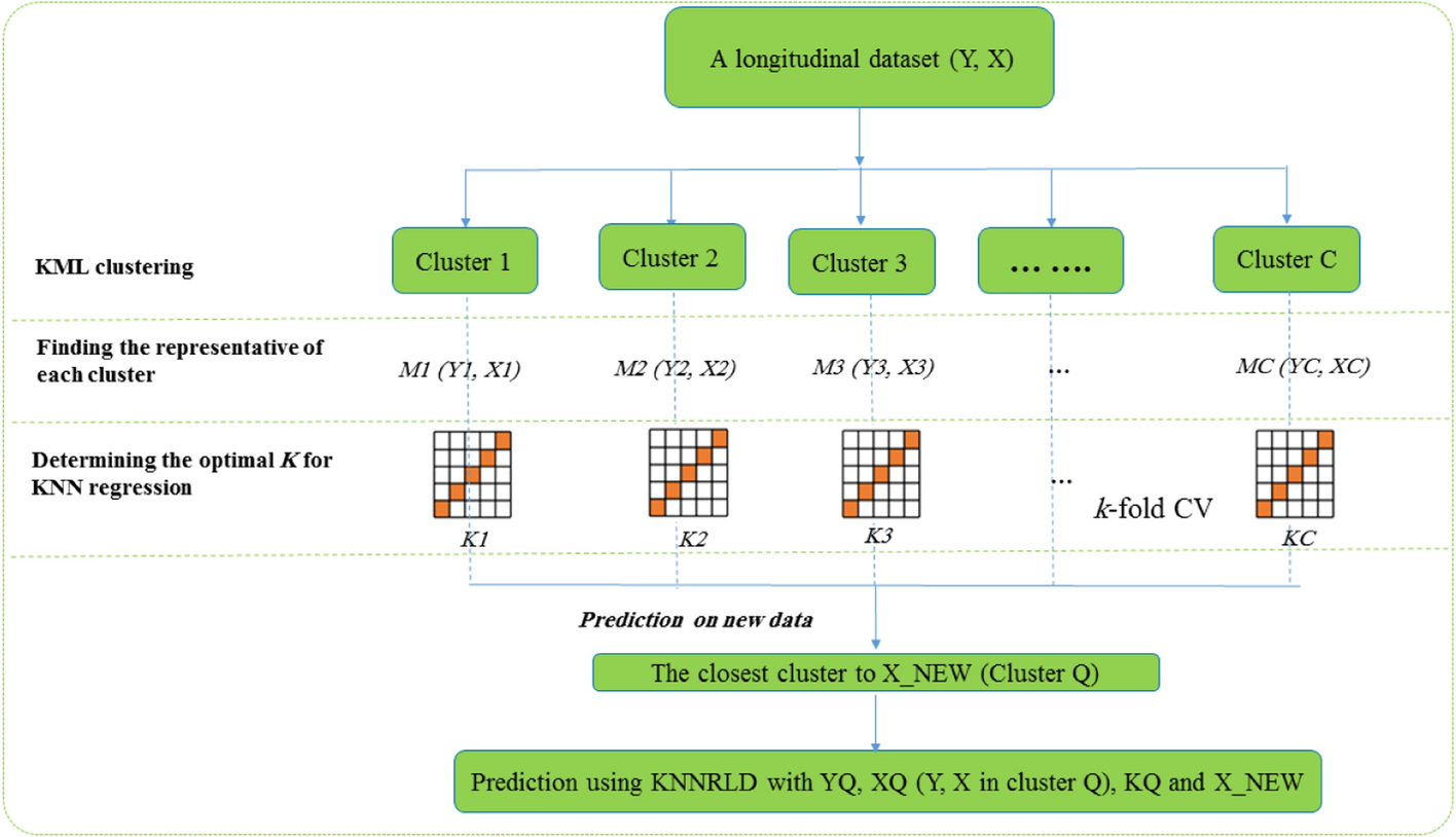
According to the above steps, the KNN regression algorithm, based on clustering for longitudinal data, is illustrated in Fig. 1. The kml package includes functions for imputing missing values, a detailed description of which is given in the related article [20]. If there are trajectories with missing values among the data, a decision can be made before step 1 with the help of the functions introduced in the kml R package. In our implementation, the optimal number of clusters was selected using internal validation indices such as the Calinski-Harabasz and silhouette scores available in the kml R package. This data-driven strategy helped ensure that the chosen C aligned with the actual data structure.
Fig. 1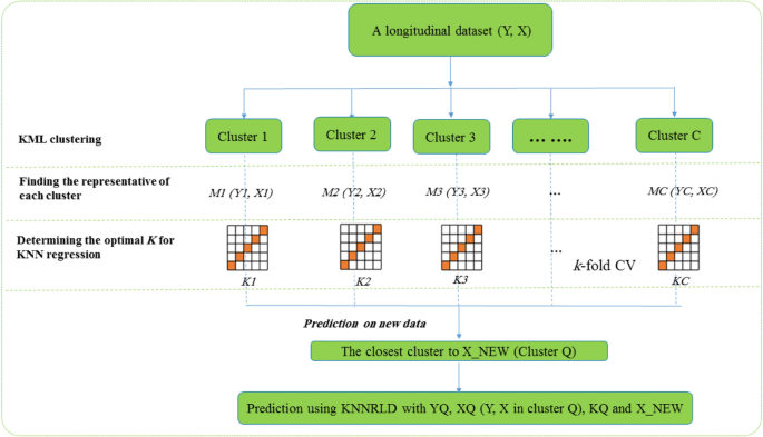
The algorithm flow plot of the CKNNLR. KNNRLD: KNN regression for Longitudinal data; CKNNRLD: clustering-Based KNN regression for longitudinal data; CV: cross-validation
Relation to previous work
CKNNRLD represents a significant advancement over existing clustering-based KNN methods by specifically addressing the unique challenges of longitudinal data analysis. While prior approaches such as CLUEKR (Dubey et al. [2]) have demonstrated the utility of combining clustering and KNN in cross-sectional settings, they lack the mechanisms necessary to handle temporal dependencies, intra-subject correlations, and irregular time points [2]. A concise comparison between CLUEKR and CKNNRLD is presented in Supplementary Table S1, summarizing key methodological differences in data type, clustering logic, and regression strategy [2].
Our method builds upon longitudinal clustering techniques, such as KML (k-means for longitudinal data), by introducing several key innovations.
Time-sensitive distance metrics: CKNNRLD employs trajectory-level distance calculations that capture both the shape and timing of individual trajectories, ensuring meaningful comparisons across subjects with sparse or irregular measurements.
Cluster-specific local regression models: By fitting regression models within clusters of similar temporal patterns, CKNNRLD adapts to heterogeneity across subgroups and improves prediction accuracy.
Scalability and flexibility: The method remains computationally efficient and non-parametric, making it suitable for large-scale longitudinal datasets without relying on strict model assumptions.
To our knowledge, no previous method has combined these components into a unified, interpretable framework for KNN-based regression on longitudinal data. Our theoretical and empirical results demonstrate that CKNNRLD offers superior performance to standard KNN approaches in terms of both accuracy and robustness in the presence of temporal complexity.
Simulation methods
The data-generating procedure first defined the number of clusters (C) that characterized the longitudinal change to be modeled into the data. Three or four clusters (C = 3, 4) with distinct longitudinal patterns (trajectories) were specified. A \(y_{ij}\) model in the general linear form below denotes a trajectory belonging to group C:
$$ y_{ij} = \beta_{0c} + \beta_{1c} t_{j} + \beta_{2jcd} X_{ijcd} + Z_{0i} + e_{ij} \;\;i = 1,…,N;j = 0,…,T $$
(18)
Here \(\beta_{oc}\), \(\beta_{1c}\) are the intercept and slope for cluster C, respectively. Furthermore, \(Z_{0i}\) it denotes the trajectory-specific random intercept; its deviation from the cluster trajectory \(Z_{0i} \sim N(0,R)\) \(e_{ij}\) represents independent random noise \(e_{ij} \sim N\;(0,E)\) In this context, tj denotes the j-th time point at which the longitudinal measurements (either for response or covariates) are observed for a given subject. In balanced data, tj can be interpreted as a fixed and common time index across subjects; in unbalanced settings, it may vary across individuals.
The simulation subsequently varied the data sets across a fixed number of repeated measurements or time points (T = 3, 5, 10) and the number of simulated subjects (N = 100, 500, 2000), which \(X_{ijcd}\) is a fictitious covariate that depends on time j and cluster c for the i-th subject. The simulation scenarios included different values for the true number of clusters (C = 3 and C = 4) to examine the model’s sensitivity to the clustering structure. The index d refers to the d-th covariate. The dimension of covariates is also considered equal to D = 2 or 3. So, the N refers to the number of subjects (or trajectories) at each time point in each cluster, yielding a total of data points in each T × C × N × D data set. For all time points and subjects error (\(e_{ij}\)) and random noise (\(Z_{0i}\)) were added to the data, taken from a normal distribution with either mean = 0 and SD = 1 (E = 1, R = 1) for the low measurement error and random noise condition, or (E = 5, R = 1), for the high measurement error and low random noise condition, or (E = 1, R = 5), for the low measurement error and high random noise condition to simulate both differences in cluster homogeneity and deviation from linearity (See Table 1).
Table 1 Summarizing the simulation scenarios
The total number of scenarios in the simulated design was 2 (clusters) × 3 (time points) × 3 (number of subjects) × 2 (dimension of covariate) × 3 (levels of error and random noise) = 108. A new series of simulated datasets was constructed for each of the three predicting methods. The number of replicated data sets per scenario was r = 10,000. The R-package latrend (Version 1.6.1) was used for this study, which can generate data according to this model using a utility function named generateLongData() included in the package [27]. This function generates datasets based on a mixture of linear mixed models (see Table 1).
Figure 2 illustrates three scenarios with common parameters, N = 500, T = 10, D = 3, and C = 4, to compare the effects of random noise and measurement error under three conditions (Fig. 2)
Fig. 2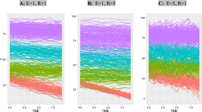
An examples of Simulated data with T = 10, D = 3, C = 4, N = 500 and E = 1, R = 1 (A panel) , E = 1, R = 5 (B panel) and E = 5, R = 1 (C panel)
The simulation study was designed to reflect the structure and conditions of the real-world longitudinal dataset analyzed in the application section. In particular, the choice of the number of covariates (D = 2 and D = 3) was motivated by the typical dimensionality observed in clinical data, where a limited number of predictors are measured repeatedly over time. Accordingly, the scenarios were constructed to mimic realistic noise levels, time structures, and clustering patterns encountered in longitudinal respiratory datasets.
The criteria for evaluating different methods for predicting new observationsAssessment of BIAS
Bias is a deviation in an estimate from the true quantity, indicating the performance of the assessed methods. One assessment of bias is the difference between the average estimate and the true value, which in this study was equal to \(BIAS = \hat{y}_{ij} – y_{ij}\) where \(\hat{y}_{ij}\) the predicted variable trajectory of the i-th person at time j is estimated using covariates under each method \(y_{ij}\) to its actual value [28].
Assessment of accuracy
The classical Mean Squared Error (MSE) is typically computed as:
$$ MSE = \frac{1}{n}\sum\limits_{i = 1}^{n} {\left( {\hat{y}_{i} – y_{i} } \right)}^{2} $$
(17)
However, in this study, a theoretical version of MSE was used to decompose the error into squared bias and variance components:
$$ Theoretical\;MSE = BIAS^{2} + SE^{2} $$
(18)
SE is the standard error, representing the empirical standard deviation of the estimator across simulations. This formulation, adapted from Burton [26], captures both systematic and random error components in the estimator’s performance [28].
Assessment of coverage probability (CP)
The coverage of a confidence interval is the proportion of times that the obtained confidence interval contains the true specified parameter value. The coverage should be approximately equal to the nominal coverage rate, e.g., 95 percent of samples for 95 percent confidence intervals, to properly control the type I error rate for testing a null hypothesis of no effect. In this study, CP refers to the proportion of times the \(100(1 – \alpha )\%\) \(\alpha = 0.05\) confidence interval \(\hat{y}_{ij} \pm Z_{{1 – \frac{\alpha }{2}}} SE\left( {\hat{y}_{ij} } \right)\) includes \(y_{ij}\), for i = 1,…, N, j = 0,…, T. If the parameter estimates are relatively unbiased, then narrower confidence intervals imply more precise estimates, suggesting gains in efficiency and power [28].
The criteria for the evaluation of clustering
We used four criteria to check the relationship between the accuracy of the estimates and the correct detection of clusters in the CKNNRLD method. Three of these are well-known criteria for evaluating the accuracy of clusters, including the Rand index [29], the Adjusted Rand index [30], and the Nowak index [31]. To calculate these three indices, the clusterSim R package (version 0.51–5) and the comparing partitions function available in this package were used [32]. In each simulation scenario, the number of clusters (C) was selected using standard internal validation indices such as the Calinski-Harabasz scores to ensure meaningful and stable clustering [26]. Moreover, one of the criteria is related to the correct detection of the algorithm in determining the number of clusters as a proportion of the matched number of clusters, which is the proportion of the number of simulation iterations in which the CKNNRLD algorithm correctly recognized the number of clusters to the total number of iterations in each simulation scenario.
Finally, Pearson’s correlation was used to assess the impact of the clustering step in the CKNNRLD algorithm on the accuracy and correctness of its estimates across all 108 scenarios.
Execution time
In the two prediction scenarios—1 predicting just one new observation and 2 predicting a random sample of observations equal to 50% of N—the execution time ratios of the KNNRLD and LMM to CKNNRLD were taken into account. These ratios were considered while comparing the execution times of the various methodologies.
Table 2 BIAS, MSE, and CP for 108 scenarios and three methodsResults on simulated data
Table 2 presents the values of BIAS, Mean Squared Error (MSE), and coverage probability (CP) related to all three CKNNRLD, KNNRLD, and LMM methods for 108 simulation scenarios.
Figure 3 compares three methods—CKNNRLD, KNNRLD, and LMM—using boxplots for bias, MSE, and CP across various simulation scenarios. LMM consistently shows higher bias and MSE, particularly as the number of clusters, time points, and error levels increase. In contrast, CKNNRLD and KNNRLD exhibit lower bias and MSE, demonstrating more stable and accurate predictions. Coverage probability is also better maintained by CKNNRLD and KNNRLD. Increasing the number of subjects reduces the mean squared error (MSE) and bias for all methods, but CKNNRLD and KNNRLD remain more robust across different conditions. Higher measurement error and random noise have a more negative impact on LMM than on the KNN approaches.
Fig. 3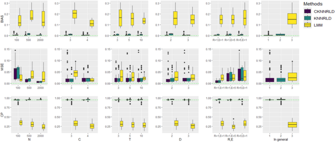
Boxplots for BIAS (top panel), MSE (middle panel), and CP (bottom panel) by simulation parameters (from left to right N, C, T, D, (R, E) and overall mean
CKNNRLD yielded lower MSE values than KNNRLD in 89.9% of scenarios, a lower bias than the LMM approach in all scenarios, and a lower MSE than the LMM approach in 65% of the scenarios (Table 2). In the CKNNRLD algorithm, an increase in the number of trajectories (N) resulted in a decrease in bias and MSE, while the CP became more consistent, approaching CP = 0.95. Conversely, the accuracy of estimates using the LMM method declined with increasing sample size (N). Similarly, the accuracy and precision of the KNNRLD approach improved as N increased, except for bias at N = 500 compared to N = 100 (Fig. 3).
The average execution time of the CKNNRLD methodology was double that of the KNNRLD method for predicting a single new longitudinal observation. In comparison, the average pure calculation time for CKNNRLD (excluding clustering timings and proximity determination for fresh data) was less than half (0.35) of the time required for the KNNRLD technique. For a random sample with fifty percent N, the average execution time ratio of the KNNRLD algorithm was less than one (0.32) in comparison to the CKNNRLD technique for N = 100; however, it was around 1.5 times (1.52) for N = 500 and roughly three times (3.04) for N = 2000 (see Fig. 4).
Fig. 4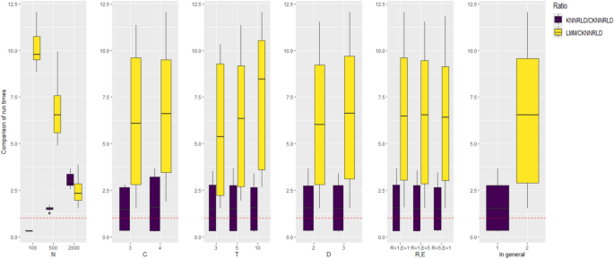
Box plots of the ratio of the run time of KNNRLD and LMM algorithms compared to CKNNRLD for fifty percent of observations as a new set of observations, by simulation parameters (from left to right N, C, T, D, (R, E) and overall mean
Supplementary Fig. S1 illustrates the sensitivity of CKNNRLD to misspecification in the number of clusters (ΔC). Specifically, it compares the mean squared error (MSE) when the true number of clusters is correctly selected (ΔC = 0) versus when C is under or overestimated by one (ΔC = ± 1). Results show that in 73% of simulation scenarios, the optimal C was selected and yielded lower MSE. In the remaining 27%, a modest increase in MSE was observed.
The Pearson correlation coefficients between clustering accuracy criteria and estimate accuracy criteria in the CKNNRLD method are presented in Table 3. The results indicate significant negative correlations between clustering accuracy indices (Rand, Adjusted Rand, and Nowak) and bias and Mean Squared Error (MSE), suggesting that improved clustering accuracy is associated with lower estimation errors. The strongest correlations are observed for the Rand index, with bias (− 0.376) and MSE (− 0.320), highlighting its relevance in ensuring precise estimation. The proportion of matched clusters also shows a weaker but significant negative correlation with bias (− 0.199) and MSE (− 0.180). However, coverage probability (CP) does not exhibit strong correlations with clustering accuracy measures, indicating that while clustering quality impacts bias and mean squared error (MSE), it has a minimal influence on the coverage of confidence intervals. These findings underscore the significance of effective clustering in enhancing the predictive performance of CKNNRLD and demonstrate that the quality of clustering has a direct impact on the regression performance of CKNNRLD. However, the method remains robust when standard validation indices are used to determine cluster structure, even in the presence of moderate noise.
Table 3 Pearson correlation of clustering accuracy criteria by estimate accuracy criteria in CKNNRLD methodApplications to real data
The severity and prognosis of respiratory diseases are primarily determined by the results of pulmonary function tests, particularly spirometry [33]. Accurate interpretation of spirometry results relies on standardized reference values that account for population-specific factors such as race, age, and height. However, respiratory scales derived from spirometry do not adhere to a linear model, as lung volumes exhibit a skewed distribution influenced by age-related and height-dependent variations. Understanding these complex patterns is crucial for precise diagnosis, monitoring disease progression, and evaluating the impact of environmental and occupational exposures on respiratory health [34,35,36,37]. Forced vital capacity (FVC) is a key indicator that reflects both restrictive and obstructive pulmonary impairments, making it essential for monitoring long-term respiratory health. Tracking changes in lung function over time is essential, particularly in occupational environments where workers may be exposed to airborne pollutants, dust, and other respiratory hazards that contribute to long-term pulmonary decline. Continuous monitoring enables the identification of early signs of impairment, facilitating timely interventions, workplace safety improvements, and the development of preventive measures to reduce the risk of chronic respiratory diseases [37, 38].
In this section, we investigate the longitudinal pattern of spirometry variables among Iran Bafq iron ore workers. The Forced Vital Capacity (FVC) variable, measured in liters, was assessed for 274 employees of this mine over three consecutive years: 2022, 2023, and 2024. Age, height, and exposure to tobacco (in pack-years; a pack-year is a clinical quantification of cigarette smoking used to measure a person’s exposure to tobacco) were considered key features. These features can be used to predict the process of changing the indicators of a new person, as they play a crucial role in determining lung function trajectories over time. Given the non-linear nature of pulmonary changes, incorporating these variables into predictive models allows for a more personalized assessment of respiratory health. By leveraging machine learning techniques, such as CKNNRLD and KNNRLD, it becomes possible to estimate future spirometry values, identify individuals at risk of lung function decline, and implement early interventions to mitigate potential respiratory impairments. For this purpose, the data were divided into two sets: train and test. The number of variable trajectories for 30 subjects (11%) was considered the test set, and the remaining data was used as the training set to train the CKNNRLD and KNNRLD methods. In Fig. 5, the variable trajectories are specified for 244 training data subjects (Panel A), and the optimal number of clusters was determined using the kml package and various criteria (see Fig. 5, Panel B). Finally, for every 30 subjects in the test dataset, the predictions from both methods and the actual values of the variable trajectories are illustrated in Panel C of Fig. 5. Internal cluster validation on the real spirometry dataset was performed using the Calinski-Harabasz criterion within the kml package. The maximum value was observed at C = 4 (CH ≈ 351.7), with C = 3 (CH ≈ 344.3) also yielding competitive scores, supporting the selection of a small number of well-separated longitudinal clusters.
Fig. 5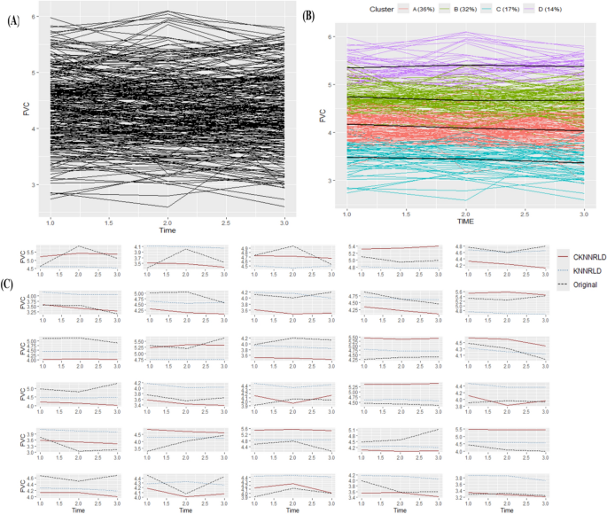
A Trajectories for training data; B KML clustering trajectory for training data; C Prediction trajectory for test data. KML, K-means for longitudinal data; FVC, forced vital capacity