
We consider a thermodynamic computer composed of N units with real-valued scalar amplitudes Si. Amplitudes could represent physical distances, if units are realized mechanically8, or voltage states, if realized by RLC circuits16,17, or phases, if realized by Josephson junctions23. The basic clock speed of the thermodynamic computer is then set by the characteristic time constants of these devices, roughly milliseconds, microseconds, or nanoseconds, respectively. Units interact via a potential V(S), which in existing thermodynamic computers consists of pairwise couplings between units16,17.
Units evolve according to the overdamped Langevin dynamics
$${\dot{S}}_{i}=-\mu \frac{\partial V({\boldsymbol{S}})}{\partial {S}_{i}}+\sqrt{2\mu {k}_{{\rm{B}}}T}\,{\eta }_{i}(t).$$
(1)
Here μ, the mobility, sets the time constant of the computer. For the thermodynamic computers described in refs. 16,17, which are realized by RLC circuits, 1/μ ∝ RC ~ 1 microsecond. The combination kBT is the thermal energy scale—kB is Boltzmann’s constant and T is temperature—and η is a Gaussian white noise with zero mean, 〈ηi(t)〉 = 0, and covariance \(\langle {\eta }_{i}(t){\eta }_{j}({t}^{{\prime} })\rangle ={\delta }_{ij}\delta (t-{t}^{{\prime} })\). The Kronecker delta δij indicates the independence of different noise components, and the Dirac delta \(\delta (t-{t}^{{\prime} })\) indicates the absence of time correlations. The noise η represents the thermal fluctuations inherent to the system. We consider the interaction V(S) and the noise η to specify the program of the thermodynamic computer.
Now say that we have a thermodynamic computer program (1) whose dynamics is slow, and so takes a long time to run (and to equilibrate, if that is our goal). The most direct way to speed up the computer is to increase the mobility parameter μ, which sets the computer’s time constant. However, for RLC circuits we do not have unlimited freedom to do this, and timescales much shorter than microseconds are difficult to arrange.
An alternative is to consider running an accelerated computer program whose solution is identical to that of the original program but which takes less time to run. We can construct such a program as follows. Rescale the interaction term V(S) by a factor λ ≥ 1—which can be done by uniformly rescaling the computer’s coupling constants, no matter how high-order in S is the potential—and introduce to the system an additional source of Gaussian white noise. Noise can be injected in a controlled way into thermodynamic computers17, single-molecule experiments24, and information engines25. If the new noise has variance σ2 then the new program is described by the equation
$${\dot{S}}_{i}=-\mu \frac{\partial [\lambda V({\boldsymbol{S}})]}{\partial {S}_{i}}+\sqrt{2\mu {k}_{{\rm{B}}}T}\,{\eta }_{i}(t)+\sigma {\zeta }_{i}(t),$$
(2)
where 〈ζi(t)〉 = 0 and \(\langle {\zeta }_{i}(t){\zeta }_{j}({t}^{{\prime} })\rangle ={\delta }_{ij}\delta (t-{t}^{{\prime} })\). The added noise ζ can be thermal (from a different heat bath) or athermal in nature, provided that it is Gaussian and has no temporal correlations. Eq. (1) assumes that the mobility μ is the same for all units. In the case of RLC circuit-based thermodynamic computers, this corresponds to all internal resistances Ri being equal (see e.g., Fig. 1 of ref. 17). This assumption does not constrain the computer’s expressive power, because its computational ability is set by the programmable inter-unit couplings V(S), not by the individual mobilities of each unit.
The two noise terms in (2) constitute an effective Gaussian white noise
$$\sqrt{2\mu {k}_{{\rm{B}}}T+{\sigma }^{2}}\,{\xi }_{i}(t),$$
(3)
where 〈ξi(t)〉 = 0 and \(\langle {\xi }_{i}(t){\xi }_{j}({t}^{{\prime} })\rangle ={\delta }_{ij}\delta (t-{t}^{{\prime} })\). If we set
$${\sigma }^{2}=2\mu {k}_{{\rm{B}}}T(\lambda -1),$$
(4)
then Eq. (2) can be written
$${\dot{S}}_{i}=-\tilde{\mu }\frac{\partial V({\boldsymbol{S}})}{\partial {S}_{i}}+\sqrt{2\tilde{\mu }{k}_{{\rm{B}}}T}\,{\xi }_{i}(t),$$
(5)
where \(\tilde{\mu }\equiv \lambda \mu\). Eq. (5) is Eq. (1) with mobility parameter rescaled by a factor λ ≥ 1 (the correlations of η and ξ are the same). Thus, the accelerated computer program (2) and (4) runs the original computer program (1) but with the clock speed increased by a factor of λ ≥ 1. (A similar effect could be achieved by rescaling V → λV and increasing temperature T → λT, but we assume that scaling temperature is less practical than adding an external source of noise.)
Another way to understand this result is to rescale time t → λt in (1): the result is Eq. (5). Put another way, Eq. (5) can be written as Eq. (1) with a modified definition of time. That is, the thermodynamics of the modified program is exactly the same as the original program: the energy barriers may be higher, but the noise is proportionally larger. As a result, the modified system evolves across this landscape in exactly the way the original system would, and samples the same equilibrium distribution. The difference is that the modified system has a redefined scale of time, and reaches its destination sooner.
For this reason the clock-rescaling trick will also work with thermodynamic computers that do calculations out of equilibrium26: the dynamical ensembles of (1) and (5) are identical, whether in or out of equilibrium. It will also work with arbitrary nonlinear interactions \({J}_{1\ldots N}{S}_{1}^{{n}_{1}}\ldots {S}_{N}^{{n}_{N}}\), because under the rescaling J1…N → λJ1…N (and the addition of noise in the correct proportion), the modified Langevin equation looks like the original Langevin equation with a rescaled time coordinate.
To illustrate this clock-acceleration procedure, we consider a classical digital simulation of the matrix inversion program of refs. 16,17. Here, the computer’s degrees of freedom possess the bilinear pairwise interaction
$$V({\boldsymbol{S}})=\sum _{\langle ij\rangle }{J}_{ij}{S}_{i}{S}_{j},$$
(6)
where the sum runs over all distinct pairs of interactions. We choose an interaction matrix Jij that is symmetric and positive definite, and so has N(N + 1)/2 distinct entries and all eigenvalues non-negative. This interaction is shown schematically in the inset of Fig. 1a. In thermal equilibrium, the probability distribution of the computer’s degrees of freedom is \({\rho }_{0}({\boldsymbol{S}})={{\rm{e}}}^{-\beta V({\boldsymbol{S}})}/\int\,{\rm{d}}{{\boldsymbol{S}}}^{{\prime} }{{\rm{e}}}^{-\beta V({{\boldsymbol{S}}}^{{\prime} })}\), where β−1 ≡ kBT, and so for the choice (6) we have \({\langle {S}_{i}\rangle }_{0}=0\) and
$${\langle {S}_{i}{S}_{j}\rangle }_{0}={\beta }^{-1}{({J}^{-1})}_{ij}.$$
(7)
Here, the brackets 〈⋅〉0 denote a thermal average, and \({({J}^{-1})}_{ij}\) denotes the elements of the inverse of the matrix J. Thus, we can invert the matrix J by sampling the thermal fluctuations, specifically the two-point correlations, of the units S in thermal equilibrium.
Fig. 1: Classical digital simulation of a thermodynamic computer program for matrix inversion16,17.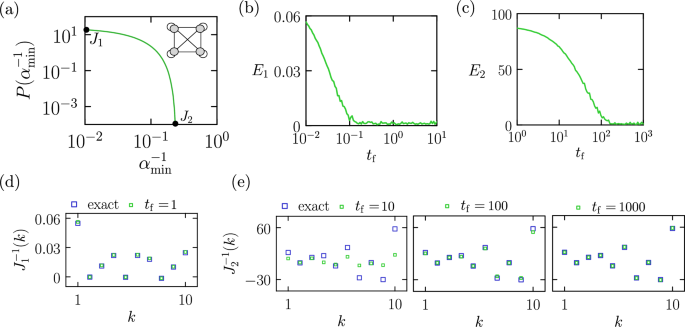
a Probability distribution of the reciprocal of the smallest eigenvalue for 107 4 × 4 symmetric positive definite matrices J. The values associated with the matrices J1 and J2 are marked by dots. Inset: schematic of the 4-unit thermodynamic computer used to estimate the inverses of J1 and J2, comprising 4 units and 10 connections. b Error E1 [Eq. (9)] in the estimate for \({J}_{1}^{-1}\) using the computer program (1) run for time tf; here and subsequently we state times in units of μ−1. The program is run ns = 104 times, from which the averages 〈SiSj〉 are calculated. c The same for the matrix \({J}_{2}^{-1}\). Note that the horizontal scales in b, c are different. d, e Estimates of the 10 distinct elements of \({J}_{1}^{-1}\) and \({J}_{2}^{-1}\), indexed by k, for the program times tf indicated. Note that the vertical axes in d, e have different scales.
We consider the case N = 4. In Fig. 1a we show the probability distribution P of the reciprocal of the smallest eigenvalue \({\alpha }_{\min }\) for 107 symmetric positive-definite 4 × 4 matrices J. These matrices were generated by first constructing random symmetric matrices B, where each distinct lower-triangular element (including the diagonal) was drawn from a Gaussian distribution with zero mean and standard deviation 0.1. We then formed the matrix A = BBT, which is guaranteed to be symmetric and positive definite. To ensure that all pairwise interaction strengths in the thermodynamic computer were of order kBT or larger, we normalized the resulting matrix by dividing all its elements by the magnitude of the smallest (in absolute value) element of A, yielding the matrix βJ. This normalization step was arbitrary and used solely for convenience. The matrix βJ is guaranteed to be positive definite, and so all its eigenvalues are positive (note that individual elements of the matrix can still be negative).
The reciprocal of the smallest eigenvalue of the matrix J provides a rough estimate of the slowest relaxation timescale of the thermodynamic computer governed by Eq. (1), when J appears in (6). The relaxation of Langevin systems with a quadratic potential can be decomposed into modes corresponding to the eigenvectors of J. Each mode relaxes exponentially, with a rate proportional to the corresponding eigenvalue27. The slowest mode, therefore, relaxes on a timescale inversely proportional to the smallest eigenvalue of J, making its reciprocal a useful proxy for the overall equilibration time. We chose two matrices, J1 and J2, whose reciprocal smallest eigenvalues are 0.011 and 0.239, respectively. Based on this metric, we expect the program defined by J2 to require at least an order of magnitude more time to equilibrate than the one defined by J1. We shall see that this expectation is borne out in a qualitative sense, although the smallest eigenvalue is not a precise predictor of the equilibration time for two-point correlations.
The matrix βJ1 is
$$\beta {J}_{1}=\left(\begin{array}{cccc}33.4484&-2.13458&-27.2213&-13.3774\\ -2.13458&91.0349&1&6.58694\\ -27.2213&1&78.3708&-12.075\\ -13.3774&6.58694&-12.075&55.602\end{array}\right),$$
and its inverse is
$${\beta }^{-1}{J}_{1}^{-1}=1{0}^{-3}\left(\begin{array}{cccc}54.806&-0.253332&21.8054&17.9513\\ -0.253332&11.0905&-0.456606&-1.47396\\ 21.8054&-0.456606&21.8886&10.0538\\ 17.9513&-1.47396&10.0538&24.6619\end{array}\right).$$
The matrix βJ2 is
$$\beta {J}_{2}=\left(\begin{array}{cccc}1.18752&1&1.00191&1.08641\\ 1&1.102484&1.02245&1.01064\\ 1.00191&1.02245&1.06828&1.03442\\ 1.08641&1.01064&1.03442&1.07344\end{array}\right),$$
and its inverse is
$${\beta }^{-1}{J}_{2}^{-1}=\left(\begin{array}{cccc}16.9091&-1.08542&11.3872&-27.0648\\ -1.08542&8.37908&-6.37593&-0.646175\\ 11.3872&-6.37593&25.497&-30.092\\ -27.0648&-0.646175&-30.092&57.9299\end{array}\right).$$
For ease of display, the matrix elements above are shown to not more than 6 significant figures.
We begin with the units of the thermodynamic computer set to zero, S = 0 (in thermal equilibrium we have 〈S〉0 = 0). We run the program (1) for time tf, and then record the value of all distinct pairwise products SiSj. To carry out these simulations we used the first-order Euler discretization of (1),
$${S}_{i}(t+\Delta t)={S}_{i}(t)-\mu \Delta t\frac{\partial V({\boldsymbol{S}})}{\partial {S}_{i}}+\sqrt{2\mu \Delta t{k}_{{\rm{B}}}T}\,X,$$
(8)
where Δt = 10−4μ−1 is the time step and \(X \sim {\mathcal{N}}(0,1)\) is a Gaussian random number with zero mean and unit variance. We set T = 1 in numerical simulations, but retain β in equations for clarity. Our simulation model runs on a conventional digital computer; when realized in hardware, the thermodynamic computer program runs automatically, driven only by thermal fluctuations.
We then reset the units of the computer to zero, and repeat the process, obtaining ns = 104 sets of measurements in all. On a single device an alternative would be to run one long trajectory and sample periodically (note that the resetting procedure could be run in parallel, if many devices are available). Using all ns = 104 samples, we compute the average 〈SiSj〉 of all distinct pairwise products. If tf is long enough for the computer to come to equilibrium, then \(\langle {S}_{i}{S}_{j}\rangle \approx {\langle {S}_{i}{S}_{j}\rangle }_{0}\) (for sufficiently large ns), and these measurements will allow us to recover the inverse of the relevant matrix via Eq. (7).
As a measure of the error E in the thermodynamic computer’s estimate of the elements \({\beta }^{-1}{({J}^{-1})}_{ij}\) we use the Frobenius norm
$$E=\sqrt{\sum _{i,j}{\left[\langle {S}_{i}{S}_{j}\rangle -{\beta }^{-1}{({J}^{-1})}_{ij}\right]}^{2}}.$$
(9)
In Fig. 1b we show the error E1 in the estimate of the inverse \({J}_{1}^{-1}\), upon using the matrix J1 in (6) and running the program (1) for time tf (in units of μ−1; subsequently, we will omit the units μ−1 when discussing timescales). For each run time, ns = 104 samples are collected. The plot indicates that thermodynamic equilibrium is attained on timescales tf ≳ 0.2.
In Fig. 1c we show the corresponding plot for the matrix J2. In this case, equilibrium is attained for run times tf ≳ 200, meaning that the run times for inverting the matrices J1 and J2 differ by about three orders of magnitude. The origin of this difference can be understood from the relative scales of the matrix elements involved: J1 encodes a thermodynamic driving force of order 10s of kBT (leading to rapid changes of S), and the associated equilibrium fluctuations of the units S are on the scale of 10−2 (which take little time to establish). By contrast, J2 encodes a thermodynamic driving force of order kBT (leading to slower changes of S), and some of the associated equilibrium fluctuations are of order 10 in magnitude (which take more time to establish).
In Fig. 1d, e we show the thermodynamic computer’s estimate of the 10 distinct matrix elements (indexed by the variable k) of \({J}_{1}^{-1}\) (panel (d)) and \({J}_{2}^{-1}\) (panel (e)), for the indicated times, upon collecting ns = 104 samples. An accurate estimate of \({J}_{2}^{-1}\) requires times in excess of 200, or of order 0.1 ms for the clock speed of the thermodynamic computer of refs. 16,17. Given that 104 samples are used, the total compute time would be of order a second, for a single 4 × 4 matrix (scaling estimates16,17 suggest that the characteristic time for matrix inversion using an overdamped thermodynamic computer will grow as the square N2 of the matrix dimension N, but matrices of equal size can have substantially different equilibration times).
To speed up the computation of \({J}_{2}^{-1}\) we can run the accelerated program specified by Eqs. (2) and (4). The matrix J2 is therefore replaced by the matrix λJ2, and we introduce an additional source of noise with variance (4). In Fig. 2a we show the error E2 in the computer’s estimate of the elements of \({J}_{2}^{-1}\), as a function of the clock acceleration parameter λ. Here, the program time is set to tf = 1, and ns = 104 samples are collected. We overlay this result on that of Fig. 1c, the error associated with the original program (1) run for time tf. As expected from comparison of (1) and (5), these results are essentially the same: the accelerated program run for tf is equivalent to the original program run for λtf.
Fig. 2: Accelerated matrix inversion program.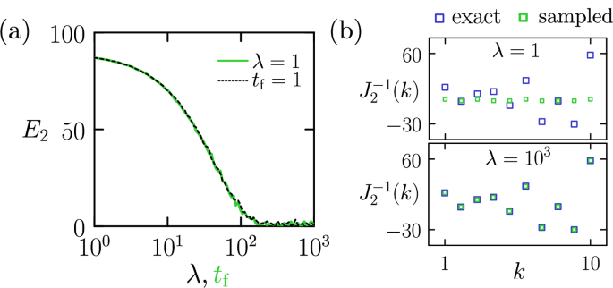
a Error E2 [Eq. (9)] in the estimate of the matrix \({J}_{2}^{-1}\) using the accelerated computer program (2) and (4) run for time tf = 1, as a function of the clock-acceleration parameter λ (black dashed line). This result is overlaid on the data of Fig. 1c, derived from the original program (1) run for time tf (green). We collect ns = 104 samples for each program. As expected from the comparison of (1) and (5), the accelerated program run for time tf is equivalent to the original program run for time λtf. b Exact elements of \({J}_{2}^{-1}\) and those estimated using the accelerated program run for time tf = 1 at two values of λ. The case λ = 1 is equivalent to the original program.
Using the accelerated program with λ = 1000, the total compute time for inverting J2 at the clock speeds of the computer of refs. 16,17 would be reduced from of order 1 s (for the original program) to of order 1 ms. If all samples were run on parallel hardware, the wall time for the computation would be of order 0.1 μs.
In panel (b), we show the inverse matrix elements extracted from the accelerated program (2) and (4) for two values of λ. As expected from the comparison of (1) and (5), the elements extracted using λ = 1000 (lower panel) for program time tf = 1 are as accurate as those extracted using the original program run for time tf = 1000 (right panel of Fig. 1e).