
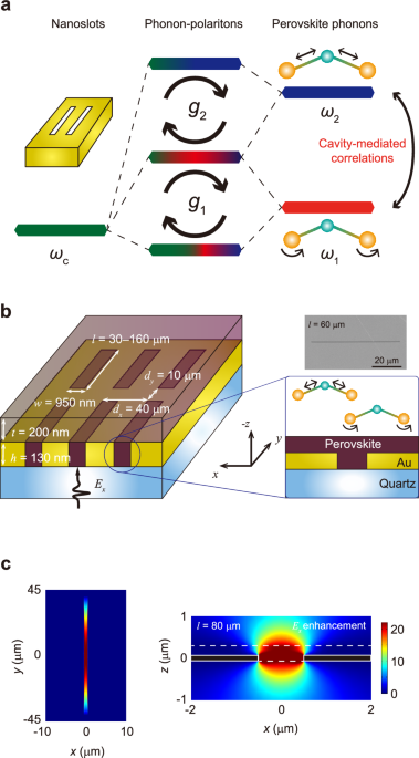
We fabricated an array of nanoslots (w = 950 nm) on quartz substrates with seven different lengths (l = 30, 40, 50, 60, 80, 120, and 160 μm) to tune the cavity mode frequency, given by \({\omega }_{{{{\rm{c}}}}}/(2\pi )={c}_{0}/(2l\sqrt{{\epsilon }_{{{{\rm{avg}}}}}})\), where c0 is the speed of light in vacuum and ϵavg = (ϵair + ϵsub)/2 represents the average dielectric constant of air and the quartz substrate (ϵsub = 2. 12)33; see Methods for sample preparation details. The resonance frequency is predominantly governed by the geometry of a single nanoslot rather than that of the periodic array34,35. Figure 1b illustrates the structure of our samples, where perovskite films (purple) are coated both on top of and within the slots.
These films exhibit two distinct optical phonon modes in free space, labeled as λ = 1 and λ = 2, corresponding to the rocking and stretching of Pb–I bonds, respectively. Due to the orientational disorder of methylammonium molecules, which breaks the lattice space-group symmetry, these phonons acquire a mixed transverse-optical (TO) and longitudinal-optical (LO) character36. As a result, they not only exhibit strong infrared absorption36,37 but also interact with lattice electrons, as recently observed5. Moreover, low-frequency phonons are particularly beneficial for achieving USC, as the normalized coupling strength g/ω increases with decreasing phonon frequency. This study, therefore, focuses on the phonons that are most relevant to strong interactions with both photonic and electronic degrees of freedom. Since electron–phonon interactions dictate charge mobility and recombination through long-range Coulomb forces, phonon-polariton formation involving low-frequency hybrid TO/LO phonons could offer effective pathways to engineer charge transport in lead halide perovskites.
Nanoslot resonators provide significant electric field enhancement due to strong optical confinement within and around the slots38,39. Since the phonon-photon coupling strength \(g\propto \sqrt{N/V}\), where N is the number of unit cells in the crystal and V is the resonator mode volume, the small mode volume of nanoslot resonators enables ultrastrong light–matter interaction regimes even with small perovskite crystals.
The in-plane spatial distribution of the cavity mode, computed using COMSOL for a perovskite-filled nanoslot, is shown in Fig. 1c (left panel). The field profile follows a sinusoidal pattern16 along the y-axis, with an electric field enhancement factor of 20 relative to transmission through a bare quartz substrate. The strong confinement of the x-component of the electric field (Ex) along the x- and z-axes results in a nearly uniform electric field within the perovskite region (Fig. 1c, right panel). Although the nanoslot thickness is 130 nm, the cavity mode extends beyond the nanoslot into the surrounding MAPbI3 layer, as depicted in Fig. 1c. The electric field strength above the nanoslot remains comparable to that inside, indicating that the perovskite film covering the slot also contributes to light–matter coupling. Notably, when t becomes comparable to the mode’s spatial extent along z, where t is the perovskite film thickness, g saturates at its maximum value; see Supplementary Note 4 and Supplementary Fig. 8.
We characterized the perovskite-nanoslot hybrid system using THz-TDS at room temperature. A normal-incident THz beam was linearly polarized along the x-axis. In free space, a 200-nm-thick MAPbI3 film exhibits transmittance dips at ω1/(2π) = 0.96 THz and ω2/(2π) = 1.9 THz, corresponding to the two phonon modes λ = 1 and λ = 2, respectively (Fig. 2a). The bare cavity resonance appears as a single peak in the transmission spectrum. Figure 2b displays the cavity resonance frequency as a function of cavity length l. By adjusting l, the cavity mode can be brought into resonance with either the λ = 1 mode (ωc = ω1) or the λ = 2 mode (ωc = ω2).
Fig. 2: Terahertz transmission spectra.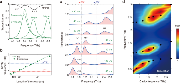
a Transmission spectra for bare cavities (nanoslots) with different lengths l (green curves) showing a single cavity mode. The green dashed line shows the simulated transmittance through the nanoslot (l = 80 μm). Transmission spectrum for a 200-nm-thick bare MAPbI3 film (black curve) showing two transmission dips due to the two optical phonon modes (λ = 1 and λ = 2) with angular frequencies ω1 and ω2, respectively. b The bare cavity resonance frequency as a function of nanoslot length l in the reciprocal axis (green circles). The linear fit (green dashed line) shows good agreement with the experimental data. The λ = 1–cavity and λ = 2–cavity resonances occur with an 80-μm-long slot and with a 50-μm-long slot, respectively, when the cavity mode frequency coincides with the phonon frequencies (red and blue dashed lines). c Transmission spectra for the MAPbI3–nanoslots hybrid system showing three polariton branches. UP upper polariton, MP middle polariton, and LP lower polariton. The dashed lines indicate the two phonon frequencies. The spectra are vertically offset by 0.2 for clarity. d Numerical simulation (COMSOL) of the transmission as a function of cavity frequency (color map). Each spectrum has been normalized by its maximum transmittance to clearly show the three polariton branches; the black solid circles are the experimental results.
Figure 2 c presents the transmission spectra of MAPbI3–nanoslot structures for different l values. As the nanoslots predominantly reflect incoming radiation, the observed polariton modes appear as transmission peaks. The spectra exhibit three distinct polariton branches: lower (LP), middle (MP), and upper (UP) polartions. These branches are separated by the uncoupled phonon modes λ = 1 and λ = 2 (dashed lines). As l decreases, the LP branch shifts toward λ = 1, the MP branch moves away from λ = 1 and approaches λ = 2, while the UP branch shifts away from λ = 2. Two anticrossings are observed at l = 80 μm and l = 50 μm, corresponding to ωc ≈ ω1 and ωc ≈ ω2, respectively (Fig. 2b). Due to the larger oscillator strength of the λ = 2 mode (Fig. 2a), the second Rabi splitting at l = 50 μm exceeds the first at l = 80 μm.
We carried out finite element simulations (COMSOL) to validate our experimental results, using conductivity values extracted from THz-TDS measurements (Supplementary Fig. 1) as input parameters. The simulated transmission spectra (Fig. 2d, colormap) closely match the experimental data, with black solid circles marking the resonance frequencies obtained from Fig. 2c via Lorentzian fitting. Minor discrepancies in the UP frequencies are attributed to slight shifts in the bare cavity mode (dashed green line, Fig. 2a) and additional coupling with a 3.8 THz phonon mode in the z-cut quartz substrate.
We also investigated a 2D perovskite material composed of metal halide layers separated by organic molecules, which enhances stability compared to 3D perovskites40,41,42 and holds promise for solar cell applications. Unlike 3D MAPbI3 (Fig. 3a), the presence of BA cations (CH3(CH2)3NH3) reduces the number of Pb-I bonds per unit volume, weakening the phonon mode oscillator strength. The layered structure, (BA)2(MA)n−1PbnI3n+1 (with n = 2)41, is shown in Fig. 3b. Here, n denotes the number of PbI6 octahedral layers between the BA spacer layers. The phonon modes λ = 1 and λ = 2 are slightly blueshifted compared to MAPbI3, with dips in the transmittance of a bare (BA)2MAPb2I7 200-nm-thick film at ω1/(2π) = 1.09 THz and ω2/(2π) = 2 THz, respectively (Supplementary Fig. 2). The transmission spectra of 2D perovskites embedded in nanoslot resonators resemble those of their 3D counterparts, with a larger Rabi splitting for λ = 2 due to its higher oscillator strength.
Fig. 3: Phonon-polariton properties in perovskite–nanoslot hybrid systems.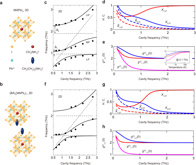
Top: MAPbI3 films (3D perovskite). Bottom: (BA)2MAPb2I7 (2D perovskite) films. a, b Crystal structures of MAPbI3 and (BA)2MAPb2I7. BA: \({{{{\rm{CH}}}}}_{3}{({{{{\rm{CH}}}}}_{2})}_{3}{{{{\rm{NH}}}}}_{3}^{+}\), MA: \({{{{\rm{CH}}}}}_{3}{{{{\rm{NH}}}}}_{3}^{+}\). c, f Polariton dispersion as a function of cavity frequency; UP upper polariton, MP middle polariton, LP lower polariton. Solid circles: Peak frequencies extracted from the experimental transmission spectra. Solid lines: Fit of the extracted peak frequencies using the microscopic Hopfield model. The dashed lines indicate the λ = 1 and λ = 2 phonon modes and the cavity resonance. The two polariton gaps (see text) are denoted as Δ1 and Δ2. d, g Phonon Hopfield coefficients (H.C.) of the LP as a function of cavity frequency, showing a divergence in the low cavity frequency limit. e, h Theoretical predictions: Equal-time second-order phonon–phonon correlation functions \({g}_{\lambda,{\lambda }^{{\prime} }}^{(2)}(\tau=0)\) for a polariton thermal state at room temperature as a function of cavity frequency. The inset in (e) shows \({g}_{\lambda,{\lambda }^{{\prime} }}^{(2)}(0)\) as a function of temperature T for a cavity frequency of 0.1 THz.
While classical electrodynamics simulations accurately reproduce the transmission spectra, we now adopt a complementary approach by utilizing a multimode Hopfield model43 to gain a deeper understanding of the ultrastrong light–matter coupling in our system and investigate its potential implications. The microscopic Hamiltonian is given by (see “Methods”)
$$\hat{H}= \hslash {\omega }_{{{{\rm{c}}}}}{\hat{a}}^{{{\dagger}} }\hat{a}+\sum\limits_{\lambda }\hslash {\omega }_{\lambda }{\hat{b}}_{\lambda }^{{{\dagger}} }{\hat{b}}_{\lambda }-i\sum\limits_{\lambda }\hslash {g}_{\lambda }\left({\hat{b}}_{\lambda }^{{{\dagger}} }-{\hat{b}}_{\lambda }\right)\left(\hat{a}+{\hat{a}}^{{{\dagger}} }\right) \\ +\sum\limits_{\lambda }\frac{\hslash {g}_{\lambda }^{2}}{{\omega }_{\lambda }}{\left(\hat{a}+{\hat{a}}^{{{\dagger}} }\right)}^{2},$$
(1)
where \({\hat{a}}^{{{\dagger}} }\) (\(\hat{a}\)) represents the creation (annihilation) operator of a cavity photon, while \({\hat{b}}_{\lambda }^{{{\dagger}} }\) (\({\hat{b}}_{\lambda }\)) denotes the creation (annihilation) operator of a phonon in the mode λ. The first two terms correspond to the bare photon and phonon Hamiltonians, respectively. The third term describes the light–matter interaction, with a coupling strength given by \({g}_{\lambda }=\frac{{\nu }_{\lambda }}{2}\sqrt{\frac{{\omega }_{\lambda }}{{\omega }_{{{{\rm{c}}}}}}}\), which is proportional to the effective ion plasma frequency νλ. The fourth term, known as the A2-term, induces a blueshift in the cavity mode frequency. The effective ion plasma frequency is determined by the effective charges associated with Pb2+ and I− ions; see “Methods” and Supplementary Note 2 for details.
The eigenfrequencies and eigenvectors of the Hamiltonian Eq. (1) are obtained via the Hopfield transformation: \({\hat{p}}_{\alpha }={\sum }_{\lambda }{X}_{\lambda,\alpha }{\hat{b}}_{\lambda }+{\sum }_{\lambda }{\widetilde{X}}_{\lambda,\alpha }{\hat{b}}_{\lambda }^{{{\dagger}} }+{Y}_{\alpha }\hat{a}+{\widetilde{Y}}_{\alpha }{\hat{a}}^{{{\dagger}} }\), where \({\hat{p}}_{\alpha }\) is the annihilation operator of a polariton in the mode α = LP, MP, UP, with frequency ωα. Up to a constant term, Eq. (1) can then be expressed in its diagonal form as \(\hat{H}={\sum }_{\alpha }\hslash {\omega }_{\alpha }{\hat{p}}_{\alpha }^{{{\dagger}} }{\hat{p}}_{\alpha }\). The system enters the USC regime when the normalized coupling strength at resonance satisfies gλ/ωλ = νλ/2ωλ ≳ 0.1. In this regime, the counter-rotating terms \(\propto {\hat{b}}_{\lambda }\hat{a},{\hat{b}}_{\lambda }^{{{\dagger}} }{\hat{a}}^{{{\dagger}} }\) in the Hamiltonian Eq. (1), along with the anomalous Hopfield coefficients \({\widetilde{Y}}_{\alpha }\) and \({\widetilde{X}}_{\lambda,\alpha }\), play a significant role.
Figure 3c presents the polariton dispersion for the MAPbI3–nanoslots system. The coupling strengths gλ are extracted by fitting the peak frequencies (solid circles) of the transmission spectra to the calculated eigenfrequencies ωα (solid lines). When the nanoslot resonator is resonant with the phonon modes λ = 1 and λ = 2, we obtain normalized coupling strengths of g1/ω1 = 0.28 (ωc = ω1) and g2/ω2 = 0.3 (ωc = ω2), respectively. These values confirm that both phonon modes are in the USC regime with the nanoslot resonator. The corresponding Rabi splittings at the two resonances are 0.45 THz and 1.13 THz. Notably, while the Rabi splitting equals exactly 2g for a single matter and cavity mode in the strong coupling regime, this relation breaks down in the USC regime due to counter-rotating terms. In our case, the inclusion of two phonon modes leads to further deviations from the 2g value. Importantly, the polariton dispersion should be understood as the result of the simultaneous coupling of both phonon modes to the cavity mode, with all three degrees of freedom treated on equal footing. This becomes evident when examining the contribution of the two phonon modes to the MP mode at around the resonance between the λ = 1 phonon and the cavity mode. As shown in Supplementary Fig. 4b, the contribution \({W}_{\lambda }^{{{{\rm{MP}}}}}=| {X}_{\lambda,{{{\rm{MP}}}}}{| }^{2}-| {\widetilde{X}}_{\lambda,{{{\rm{MP}}}}}{| }^{2}\) of the two phonon modes (λ = 1, 2) to the MP mode is indeed of comparable magnitude, indicating that the MP branch involves significant hybridization with both phonon modes.
In the USC regime, distinctive features appear not only near resonance, but also when the resonator frequency is much lower than the phonon frequencies, ωc ≪ ωλ. Unlike in the strong coupling regime, the polariton modes do not converge to the uncoupled mode frequencies when ωc ≪ ωλ. This behavior defines the so-called polariton gaps19,44, given by \({\Delta }_{1}={\lim }_{{\omega }_{{{{\rm{c}}}}}\to 0}{\omega }_{{{{\rm{MP}}}}}-{\omega }_{1}\) and \({\Delta }_{2}={\lim }_{{\omega }_{{{{\rm{c}}}}}\to 0}{\omega }_{{{{\rm{UP}}}}}-{\omega }_{2}\), as shown in Fig. 3c. As detailed in Supplementary Note 3, the frequencies of the MP and UP modes, ωMP and ωUP, asymptotically approach \({\widetilde{\omega }}_{1}=\sqrt{{\omega }_{1}^{2}+{\nu }_{1}^{2}}\) and \({\widetilde{\omega }}_{2}=\sqrt{{\omega }_{2}^{2}+{\nu }_{2}^{2}}\), respectively, in the low-resonator frequency limit ωc → 0.
This unconventional behavior is linked to strong light–matter hybridization, which persists even in this far-detuned, low-resonator-frequency regime. This is reflected in the divergence of the light–matter coupling strength, \({g}_{\lambda }\propto \sqrt{1/{\omega }_{{{{\rm{c}}}}}}\), and the A2-term, which scales as \({g}_{\lambda }^{2}\), as ωc → 0. In this regime, the MP (UP) mode is mainly a hybrid of the phonon mode λ = 1 (λ = 2) and cavity photons. The corresponding normal (Yα) and anomalous (\({\widetilde{Y}}_{\alpha }\)) Hopfield coefficients become large and comparable, scaling as \({Y}_{{{{\rm{MP}}}}} \sim {\widetilde{Y}}_{{{{\rm{MP}}}}} \sim {\nu }_{1}/\sqrt{{\omega }_{{{{\rm{c}}}}}{\widetilde{\omega }}_{1}}\) and \({Y}_{{{{\rm{UP}}}}} \sim {\widetilde{Y}}_{{{{\rm{UP}}}}} \sim {\nu }_{2}/\sqrt{{\omega }_{{{{\rm{c}}}}}{\widetilde{\omega }}_{2}}\). In contrast, the LP mode mixes the cavity field with both phonon modes. The phonon contributions to this polariton, quantified by the coefficients Xλ,LP and \({\widetilde{X}}_{\lambda,{{{\rm{LP}}}}}\), also grow large and comparable, with \({X}_{\lambda,{{{\rm{LP}}}}} \sim {\widetilde{X}}_{\lambda,{{{\rm{LP}}}}} \sim {\nu }_{\lambda }/\sqrt{{\omega }_{{{{\rm{c}}}}}{\omega }_{\lambda }}\). These coefficients are shown in Fig. 3d, while the other Hopfield coefficients are provided in Supplementary Figs. 3 and 5.
Due to the large anomalous Hopfield coefficients, the polaritonic ground state \(\left\vert G\right\rangle\), defined by \({\prod }_{\alpha }{\hat{p}}_{\alpha }\left\vert G\right\rangle=0\), takes the form of a multimode squeezed vacuum in the low resonator frequency regime. This state contains correlated photon pairs, contributed by the MP and UP, as well as intermode and intramode phonon pairs originating from the LP. This multimode squeezed vacuum exhibits strong entanglement between the two phonon modes, as discussed below.
It is important to highlight that while both the normal and anomalous Hopfield coefficients diverge in the limit ωc → 0, the total phonon and photon weights remain finite due to the normalization of the Hopfield coefficients (see Supplementary Figs. 4 and 6). Moreover, we stress that the low-resonator-frequency regime (long cavity) does not imply the absence of a cavity, as its transverse confinement remains deeply subwavelength.
A distinctive feature of the multimode USC regime is the presence of anomalous correlations between the phonon modes. By inverting the Hopfield transformation, one obtains the correlation functions:
$$\langle {\hat{b}}_{\lambda }^{{{\dagger}} }{\hat{b}}_{{\lambda }^{{\prime} }}\rangle=\sum\limits_{\alpha }{\left({\widetilde{X}}_{\lambda }^{\alpha }\right)}^{*}{\widetilde{X}}_{{\lambda }^{{\prime} }}^{\alpha }(1+{n}_{\alpha })+\sum\limits_{\alpha }{X}_{\lambda }^{\alpha }{\left({X}_{{\lambda }^{{\prime} }}^{\alpha }\right)}^{*}{n}_{\alpha },$$
(2)
$$\langle {\hat{b}}_{\lambda }{\hat{b}}_{{\lambda }^{{\prime} }}\rangle=-\sum\limits_{\alpha }{\left({X}_{\lambda }^{\alpha }\right)}^{*}{\widetilde{X}}_{{\lambda }^{{\prime} }}^{\alpha }(1+{n}_{\alpha })-\sum\limits_{\alpha }{\left({X}_{{\lambda }^{{\prime} }}^{\alpha }\right)}^{*}{\widetilde{X}}_{\lambda }^{\alpha }{n}_{\alpha }.$$
(3)
Here, \({n}_{\alpha }=\langle {\hat{p}}_{\alpha }^{{{\dagger}} }{\hat{p}}_{\alpha }\rangle\) represents the population in the polariton mode α. In the polaritonic ground state (nα = 0), Eqs. (2) and (3) show that such correlations arise only when the anomalous Hopfield coefficients \({\widetilde{X}}_{\lambda }^{\alpha }\) are nonzero. Moreover, these correlations are further enhanced in excited polariton states where nα ≠ 0. To explore the impact of multimode USC on correlated phonon emission, we consider the second-order correlation function45, which quantifies the joint probability of a phonon being emitted in the mode \({\lambda }^{{\prime} }\) at time t + τ given that a phonon was emitted in the mode λ at time t:
$${g}_{\lambda,{\lambda }^{{\prime} }}^{(2)}(\tau )=\frac{\langle {\hat{b}}_{{\lambda }^{{\prime} }}(t+\tau ){\hat{b}}_{\lambda }(t){\hat{b}}_{\lambda }^{{{\dagger}} }(t){\hat{b}}_{{\lambda }^{{\prime} }}^{{{\dagger}} }(t+\tau )\rangle }{\langle {\hat{b}}_{\lambda }(t){\hat{b}}_{\lambda }^{{{\dagger}} }(t)\rangle \langle {\hat{b}}_{{\lambda }^{{\prime} }}(t+\tau ){\hat{b}}_{{\lambda }^{{\prime} }}^{{{\dagger}} }(t+\tau )\rangle }.$$
(4)
Although classical wave-based methods could, in principle, be used to study intensity correlations, such calculations are technically challenging and non-trivial to implement. For this reason, we focus in this work on quantum predictions for the second-order correlation functions. Assuming a thermal polariton state at temperature T, with \({n}_{\alpha }={\left({e}^{\hslash {\omega }_{\alpha }/{k}_{{{{\rm{B}}}}}T}-1\right)}^{-1}\) and kB the Boltzmann constant, the equal-time intramode (\(\lambda={\lambda }^{{\prime} }\)) and intermode (\(\lambda \, \ne \, {\lambda }^{{\prime} }\)) correlation functions are given by
$${g}_{\lambda,\lambda }^{(2)}(0)=2+\frac{\langle {\hat{b}}_{\lambda }{\hat{b}}_{\lambda }\rangle \langle {\hat{b}}_{\lambda }^{{{\dagger}} }{\hat{b}}_{\lambda }^{{{\dagger}} }\rangle }{{\langle {\hat{b}}_{\lambda }{\hat{b}}_{\lambda }^{{{\dagger}} }\rangle }^{2}},$$
(5)
$${g}_{\lambda,{\lambda }^{{\prime} }}^{(2)}(0)=1+\frac{\langle {\hat{b}}_{\lambda }{\hat{b}}_{{\lambda }^{{\prime} }}^{{{\dagger}} }\rangle \langle {\hat{b}}_{{\lambda }^{{\prime} }}{\hat{b}}_{\lambda }^{{{\dagger}} }\rangle }{\langle {\hat{b}}_{\lambda }{\hat{b}}_{\lambda }^{{{\dagger}} }\rangle \langle {\hat{b}}_{{\lambda }^{{\prime} }}{\hat{b}}_{{\lambda }^{{\prime} }}^{{{\dagger}} }\rangle }+\frac{\langle {\hat{b}}_{\lambda }{\hat{b}}_{{\lambda }^{{\prime} }}\rangle \langle {\hat{b}}_{{\lambda }^{{\prime} }}^{{{\dagger}} }{\hat{b}}_{\lambda }^{{{\dagger}} }\rangle }{\langle {\hat{b}}_{\lambda }{\hat{b}}_{\lambda }^{{{\dagger}} }\rangle \langle {\hat{b}}_{{\lambda }^{{\prime} }}{\hat{b}}_{{\lambda }^{{\prime} }}^{{{\dagger}} }\rangle },$$
(6)
respectively. For vanishing anomalous Hopfield coefficients (\({\widetilde{X}}_{\lambda }^{\alpha }=0\,\forall \lambda\)) or in the absence of phonon–photon coupling (νλ = 0), Eq. (5) simplifies to \({g}_{\lambda,\lambda }^{(2)}(0)=2\), which corresponds to intramode phonon bunching-a hallmark of thermal states. In contrast, the intermode correlation function satisfies \({g}_{\lambda,{\lambda }^{{\prime} }}^{(2)}(0)=1\) for \(\lambda \, \ne \, {\lambda }^{{\prime} }\), indicating that intermode phonon emission remains uncorrelated and follows Poissonian statistics46.
In the multimode USC regime, we predict a significant modification of equal-time phonon-phonon second-order correlations. As shown in Fig. 3e, the various contributions \({g}_{\lambda,{\lambda }^{{\prime} }}^{(2)}(0)\) to a value of 3 in the limit of a vanishing resonator frequency (ωc → 0). As ωc increases, \({g}_{\lambda,{\lambda }^{{\prime} }}^{(2)}(0)\) decreases monotonically, approaching 2 for intramode correlations (\(\lambda={\lambda }^{{\prime} }\)) and 1 for intermode correlations (\(\lambda \ne {\lambda }^{{\prime} }\)). These limiting values correspond to the correlations expected for bare phonons, which are recovered in the high resonator frequency regime (ωc ≫ ωλ), where the LP and MP asymptotically approach the uncoupled phonon frequencies ω1 and ω2, respectively.
For a detuned cavity with ωc/(2π) = 0.1 THz at room temperature (T = 300 K), our theoretical model predicts \({g}_{1,1}^{(2)}(0)\approx 2.86\), \({g}_{2,2}^{(2)}(0)\approx 2.96\), and \({g}_{1,2}^{(2)}(0)\approx 2.82\). These results indicate that multimode USC should lead to strong phonon bunching in both intramode and intermode correlations. This effect primarily arises from the LP, which exhibits large normal and anomalous phonon Hopfield coefficients (\({X}_{\lambda }^{\alpha },{\widetilde{X}}_{\lambda }^{\alpha }\)), as discussed earlier, along with a significant population in the low resonator frequency regime (nLP ≈ 80 for ωc/(2π) = 0.1 THz and T = 300 K). The inset of Fig. 3e illustrates the temperature dependence of the calculated second-order phonon correlations, showing that at T = 0 K, intramode and intermode correlations are enhanced by approximately 10% and 40%, respectively, compared to the bare phonon case. Notably, at room temperature, \({g}_{\lambda,{\lambda }^{{\prime} }}^{(2)}(0)\) remains in the saturation regime.
Figure 3f presents the extracted peak frequencies for the 2D perovskite (BA)2MAPb2I7–nanoslots system, alongside theoretical predictions (solid lines). In this case, the λ = 1 mode exhibits a very small polaritonic gap, which is consistent with the normalized coupling strength \({g}_{1}^{{\prime} }/{\omega }_{1}=0.13\) extracted from the fit. This value suggests that λ = 1 is on the verge of the USC regime, leading to reduced Hopfield coefficients X1,LP and \({\widetilde{X}}_{{{{\rm{1,LP}}}}}\) compared to the MAPbI3–nanoslots system (see Fig. 3g). Conversely, the polaritonic gap of the λ = 2 mode remains similar to that observed in the MAPbI3–nanoslots system, consistent with the large coupling ratio \({g}_{2}^{{\prime} }/{\omega }_{2}=0.23\) extracted from the fit.
At ωc/(2π) = 0.1 THz and room temperature, the calculated phonon-phonon correlations for \(\lambda={\lambda }^{{\prime} }=1\) and \(\lambda=1,{\lambda }^{{\prime} }=2\) are significantly lower than in the MAPbI3-nanoslots system (\({g}_{1,1}^{(2)}(0)\approx 2.61\), \({g}_{1,2}^{(2)}(0)\approx 2.52\)), in line with the weaker coupling strength of λ = 1. However, \({g}_{2,2}^{(2)}(0)\approx 2.94\) remains nearly unchanged compared to the 3D perovskite system, as shown in Fig. 3h.
Using a perturbative expansion valid for ωc/ωλ ≪ 1 and νλ/ωλ ≪ 1, we show in Supplementary Note 3 that the second-order correlation functions can be approximated as
$${g}_{1,1}^{(2)}(0)\approx 2+{\left(\frac{{g}_{1}}{{\omega }_{1}}\right)}^{4}{\left(\frac{1+2{n}_{{{{\rm{LP}}}}}}{1+{n}_{{{{\rm{MP}}}}}}\right)}^{2}$$
(7a)
$${g}_{2,2}^{(2)}(0)\approx 2+{\left(\frac{{g}_{2}}{{\omega }_{2}}\right)}^{4}{\left(\frac{1+2{n}_{{{{\rm{LP}}}}}}{1+{n}_{{{{\rm{UP}}}}}}\right)}^{2}$$
(7b)
$${g}_{1,2}^{(2)}(0)\approx 1+2{\left(\frac{{g}_{1}}{{\omega }_{1}}\right)}^{2}{\left(\frac{{g}_{2}}{{\omega }_{2}}\right)}^{2}\frac{{(1+2{n}_{{{{\rm{LP}}}}})}^{2}}{(1+{n}_{{{{\rm{MP}}}}})(1+{n}_{{{{\rm{UP}}}}})}.$$
(7c)
These results show that the intramode correlation functions are primarily controlled by the standard USC figure of merit, gλ/ωλ. In contrast, intermode correlations are governed by the product g1g2/ω1ω2, which becomes an important figure of merit for multimode USC. For instance, we find g1g2/ω1ω2 = 0.084 in the 3D perovskite-nanoslot system and g1g2/ω1ω2 = 0.03 in the 2D system. The specific form g1g2/ω1ω2 suggests that intermode correlations arise from the effective coupling between phonons mediated by the far-detuned cavity, where ωc ≪ ωλ.