SpatPPI: a geometric deep learning model for predicting protein–protein interactions involving intrinsically disordered regions | Genome Biology

Data preparation

In this section, we introduce the details of the datasets used in this study, including the selection of intrinsically disordered regions, the creation of the HuRI-IDP dataset, an overview of the STRING11.0 human dataset [36], and the construction of the novel protein test set (see Table 1 for an overview of the datasets used in the study).

Table 1 Overview of the datasets used in this study

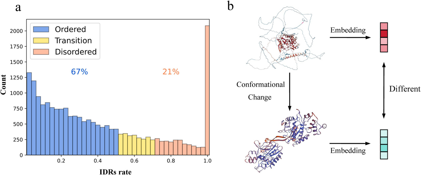
Selection of intrinsically disordered regions. Previous studies have shown that regions of low confidence in AlphaFold2 predictions are highly consistent with IDRs [37]. Window-averaged AlphaFold2 pLDDT scores can be an effective tool for predicting IDRs. Specifically, residues with pLDDT > 0.8, pLDDT < 0.7, and 0.7 ≤ pLDDT ≤ 0.8 were first labeled as folded, disordered, and gap regions, respectively. Next, folded and disordered regions shorter than ten residues were reclassified as gap regions. If a gap region (i) was surrounded by disordered regions or (ii) was located at the termini with adjacent disordered regions, it was relabeled as disordered. All other gap regions were relabeled as folded regions. Additionally, since AlphaFold2 sometimes assigns high pLDDT scores to certain residues in known IDRs, possibly related to specific conditions such as binding or post-translational modifications, we also referred to Tesei’s approach and used SPOT-Disorder v.1 to identify IDRs [38]. In this study, the concatenation of the prediction results of these two prediction methods was used as the final IDRs region.

HuRI-IDP dataset. To evaluate the performance of SpatPPI in predicting IDPPI, we used the data from the HuRI Mapping Project, which detected 52,569 PPIs involving 8727 human proteins through high-throughput yeast two-hybrid screens. This project is both comprehensive and reliable, and importantly, it includes a higher proportion of intrinsically disordered proteins among the proteins involved, which facilitated the construction of our IDPPI dataset.

We define proteins with IDRs accounting for more than 70% of their total residues as intrinsically disordered proteins, those with IDRs accounting for less than 50% as structurally stable proteins, and the remainder as transitional proteins. To minimize the impact of sequence similarity, we used CD-HIT [39, 40] to cluster the protein sequences, setting a sequence identity threshold of 40%. After stringent sequence similarity filtering, 6831 proteins remained.

In this study, IDPPI refers to a PPI between an intrinsically disordered protein and a structurally stable protein. In the training set and test set A, IDPPI does not include transitional proteins. However, in test set B, due to the limited availability of proteins, approximately 10% of IDPPI pairs involve transitional proteins and structurally stable proteins. Our IDPPI training set contains 2800 positive and 28,000 negative protein interactions, with IDPPI accounting for 50% of both positive and negative samples. Test set A comprises 200 positive sample pairs (100 IDPPI) and 2000 negative sample pairs, while test set B contains 300 positive sample pairs (200 IDPPI) and 3000 negative sample pairs. The difference between them is that test set A was randomly divided along with the training set (ensuring an IDPPI proportion of 50%), with 95% of the proteins appearing in the training set, while test set B was constructed separately to ensure that the intrinsically disordered proteins had never appeared in the training set. For test set B construction, positive samples were rigorously curated to preferentially include IDRs with manually annotated disorder status, thereby mitigating the risk of misclassifying conventional PPIs as IDPPIs. All positive samples in the datasets were derived from the HuRI Mapping Project, with the exception of approximately 20% of positive samples in test set B, which originated from the STRING database. The number of negative samples is 10 times higher than that of positive samples, and each negative sample is randomly paired from all proteins [41]. Additionally, we introduced 10,000 extra proteins to generate negative samples, ensuring that no protein appeared too many times in the training set.

STRING11.0 human dataset. To verify the generalization performance of SpatPPI, we trained a new SpatPPI model using the same dataset as D-SCRIPT and Topsy-Turvy. The positive interactions in this dataset were extracted from the STRING v11 database, which covers various PPI networks and integrates comprehensive information from multiple major sources. The protein sequences in this dataset range from 50 to 800 amino acids in length, and the sequence similarity between protein pairs is strictly controlled below 40% to avoid the model over-relying on sequence similarity when predicting interactions. To better reflect the naturally observed frequency of positive interactions, the ratio of positive to negative samples in the D-SCRIPT dataset was set at 1:10. Negative interactions were generated by randomly pairing different proteins from the non-redundant interaction set.

Novel protein test set. The AlphaFold Protein Structure Database (AFDB) initially provided 23,391 predicted human protein structures (https://ftp.ebi.ac.uk/pub/databases/alphafold/latest/UP000005640_9606_HUMAN_v4.tar). We applied a chain length filter (50–2000 residues) to exclude fragments and oversized assemblies, yielding a subset of 20,487 proteins. These structures were further processed through CD-HIT clustering with a 60% sequence similarity threshold, resulting in 16,576 non-redundant clusters. After removing proteins that appeared in the STRING11.0 human dataset, 1500 protein structures remained. We used these 1500 proteins to construct the novel protein test set. The STRING v12 database [42] contains richer protein interaction data than STRING v11. We queried the STRING v12 database for interaction data within the novel protein set, selecting 200 high-confidence interactions with a combined score greater than 0.90 as positive samples for the novel protein test set. For negative samples, we used an intra-group pairing strategy, generating 2000 pairs of negative samples while limiting each protein to participate in no more than six negative sample pairs to ensure diversity and validity.

The SpatPPI architecture

In this section, we provide a detailed description of the SpatPPI model framework, which comprises four main components: graph representation of protein structures, feature extraction, graph self-attention aggregation with conformation reorganization, and residue contact capture module.

1) Graph representation of protein structures.

The complex topological structure of proteins makes feature extraction more challenging compared to protein sequences. A common strategy involves converting protein structures into graphs (Additional file 2: Fig. S4). Given a protein P, SpatPPI constructs the graph in two stages: first, an undirected graph Gᵤ is built where nodes represent amino acid residues, with each node connected to its k nearest spatial neighbors based on Euclidean distance. Specifically, SpatPPI uses Cα atom coordinates to represent spatial positions. The pairwise Euclidean distances between residues are computed to generate a distance matrix, from which the k smallest values (excluding diagonal zeros) are selected row-wise to establish edges between corresponding nodes.

Subsequently, local coordinate systems are established for each residue. The 20 common amino acids have a general structural formula. The carbon atom directly connected to the carboxyl group is called the Cα, and R represents the side chain group, which determines the properties and functions of the amino acid. We considered the orientation of the side chain group in space to be of significant importance in characterizing the property distribution of the protein chain [43,44,45]. Therefore, to clearly represent the spatial property distribution, a coordinate system Oi was built for each amino acid residue as follows:

$$\begin{array}{c}{O}_{i}=\left[{f}_{i1},{f}_{i2},{f}_{i3}\right]\end{array},$$

$${f}_{i3}\left(zaxis\right)=\frac{{x}_{iSCoM}-{x}_{{iC}_{\alpha }}}{||{x}_{iSCoM}-{x}_{{iC}_{\alpha }}||},$$

$${f}_{i2}\left(yaxis\right)=\frac{{f}_{i3}\times \left({x}_{{iC}_{\alpha }{\prime}}-{x}_{i{C}_{\alpha }}\right)}{||{f}_{i3}\times \left({x}_{{iC}_{\alpha }{\prime}}-{x}_{i{C}_{\alpha }}\right)||},$$

$${f}_{i1}\left(xaxis\right)=\frac{{f}_{i3}\times {f}_{i2}}{|\left|{f}_{i3}\times {f}_{i2}\right||},$$

where \(\times\) denotes the cross-product. The Cα was set as the origin of the coordinate system, and the line connecting the Cα to the side chain centers of mass (SCoM) is taken as the z-axis. Additionally, the normal vector of the plane formed by the Cα, SCoM, and the Cα of the previous amino acid residue (C′α) is defined as the y-axis direction, constructing a right-handed right-angle Cartesian coordinate system.

The undirected graph Gᵤ is then traversed to convert edges into directed ones by treating each node as tail and its neighbors as heads. The seven-dimensional edge attributes eij are all calculated based on the local coordinate system. The first three dimensions are the spatial coordinates of other nodes j in the current node’s i coordinate system, reflecting the spatial positional information between residues. The 4th to 7th dimensions from a quaternion, representing the rotation matrix of the coordinate system of other nodes within the current node’s coordinate system, reflecting the orientation information of the side chain group of residues (Additional file 1: Note S5). The specific method for quaternion conversion is the same as in Fang et al. [46, 47]. After removing original undirected edges, we obtain the final directed graph G with multidimensional edge attributes.

$${e}_{ij}=\left({O}_{i}^{T}\frac{{x}_{j{C}_{\alpha }}-{x}_{i{C}_{\alpha }}}{\Vert {x}_{j{C}_{\alpha }}-{x}_{i{C}_{\alpha }}\Vert },q\left({O}_{i}^{T}{O}_{j}\right)\right).$$

During the conversion of the protein into a graph, all residue attribute information is concentrated in the nodes, while the information needed to determine the spatial orientation between residues is concentrated in the edges. The independence of these two elements makes it possible to achieve adjustments to the protein structure within the model.

2) Feature extraction.

SpatPPI extracts 41-dimensional amino acid features V for each amino acid residue in a protein. Dimensions 1–20 represent the sequence evolutionary features of the amino acid residues, dimensions 21–33 represent structural features including secondary structure information and backbone torsion angles, dimension 34 represents the hydrophobicity feature, and dimensions 35–41 represent the physicochemical properties of the amino acid residues detailed as follows.

Sequence evolutionary features. The Position-Specific Scoring Matrix (PSSM) provides conservation information for amino acid residues and is commonly used in PPI prediction tasks. It represents the likelihood of each amino acid appearing at every position in a protein’s amino acid sequence. In this study, the PSSM matrix was generated using the PSI-BLAST with three iterations and an e value parameter of 0.001, searching the Uniref50 database [48, 49]. We used only the first 20 columns of the PSSM matrix, corresponding to the 20 common amino acids. The value in the i row and j column reflects the probability that the amino acid at position i will mutate to the j amino acid during evolution; the higher the value, the greater the probability. Before computation, each element x in the PSSM is normalized to the range [0,1] by a sigmoid function:

$$\overline{x}=\frac{1}{1+{e}^{-x}}.$$

Secondary structure profile. SpatPPI used a 13-dimensional vector to represent the structural features of an amino acid, with the first 8 dimensions representing 8 possible states of secondary structure, and the remaining 5 dimensions representing bond angles and torsion angles. The DSSP, based on classical hydrogen bond detection, is the most widely used secondary structure definition system [50, 51]. In DSSP, protein secondary structure is categorized into three major classes—helix, sheet, and loop. The helix class includes α-helix, 310-helix, and π-helix; the sheet class includes extended strand and \(\beta\)-bridge; and the loop class includes hydrogen-bonded turns, bends, and irregular loops, totaling 8 subclasses.

Solvent accessibility feature. Solvent accessibility reflects the surface area of an amino acid residue that can contact solvent molecules. Since protein–protein interactions typically occur on or near the surface of proteins, the solvent exposure of amino acid residues is also useful information for PPI prediction. In this study, the ratio of the current solvent-accessible surface area of a residue to its maximum solvent-accessible surface area is used as an indicator of its solvent accessibility, which can also be extracted from the DSSP file.

Atomic features of residues. For a residue, we extracted seven features for each atom belonging to that residue (excluding hydrogen atoms), including atom mass, B-factor, whether the atom is a side-chain atom, electronic charge, number of bonded hydrogen atoms, whether the atom is in a ring, and Van der Waals radius of the atom. Since different amino acid residues have varying numbers of atoms, SpatPPI takes the average of the corresponding features of all atoms as the value of that feature for the amino acid residue.

3) Graph self-attention aggregation for conformation reorganization.

Using graphs to represent protein structures is a common approach. In past studies, many graph network models, including graph convolutional networks (GCN), graph attention networks (GAT), and graph isomorphism networks (GIN), have been applied to PPI prediction tasks that integrate structural information. In these methods, the node embeddings, which represent the residue entity features, have been well-learned. However, the edge embeddings, which represent the spatial conformation between residues, have not received sufficient attention [52]. Here, we modify the graph attention network framework to compute the attention coefficient αij between any two nodes i and j as follows:

$${\alpha }_{ij}=\text{softmax}\left(\frac{{\left({W}_{Q}{V}_{i}\right)}^{T}\left(\left({W}_{{K}_{1}}{V}_{j})\odot({W}_{{K}_{2}}{e}_{ij}\right)\right)}{d}\right),$$

where Vi and Vj are the hidden embeddings of node i and node j, respectively, and eij is the edge embedding from node i to node j. WQ, WK1, and WK2 are learnable weight matrices used to project the embeddings to the query and double key embeddings. d represents the hidden dimension. \(\odot\) denotes Hadamard (element-wise) product. Contrary to conventional self-attention mechanisms, we employ two matrices to disentangle edge information from node information. Our aim is to amplify the impact of edge features during node aggregation, thereby ensuring that a residue pair is assigned greater aggregation weights solely when they exhibit both suitable spatial conformations and complementary entity characteristics. Consequently, the formula for aggregating node embeddings can be formulated as follows:

$${V}_{i}{\prime}={V}_{i}+{\sum }_{j\epsilon N\left(i\right)}{\alpha }_{ij}{W}_{v}\left(\left[{V}_{j} || {e}_{ij}\right]\right),$$

where || represents the vector concatenation operation, and N(i) denotes the set of k neighboring nodes of node i. Wv is learnable weight matrix.

The predicted structures stored in the AlphaFold Protein Structure Database have unique structural characteristics in their IDRs: these regions exhibit homogeneity in secondary structure, and the residues maintain relatively stable spatial relationships within their k-order neighborhoods. Since IDRs and structurally stable regions are continuously distributed in sequence, and node aggregation occurs within local neighborhoods, this operation enhances the distinction between IDR node embeddings and those of structurally stable regions. To ensure that this distinguishability is not averaged out during multi-layer graph aggregation, we update the edge embeddings with new node embeddings after each node aggregation:

$${e}_{ij}{\prime}=MLP\left(\left[{V}_{i}{\prime}\Vert {e}_{ij}\Vert {V}_{j}{\prime}\right]\right).$$

The edge embeddings are initially defined by the spatial relative position and orientation between amino acid residues. Updating them essentially reconstructs the original protein in space. This process is designed to preserve and enhance the uniqueness of inter-regional connections while integrating information from folded domains into the structural updates of adjacent IDRs. It ensures that the dynamic structural characteristics of IDRs are effectively retained throughout the message passing process of the complex graph neural network.

4) Residue contact capture module.

The graph neural network generates representations for each residue of any given protein, forming a residue representation matrix. However, to obtain the interaction probability between proteins, it is necessary to enable residue contact capture between the two proteins.

Assuming that the final output of the graph aggregation layer generates residue embedding matrices X ∈ Rφ×m and Y ∈ Rφ×n for the two proteins in any sample pair, where m and n denote the number of residues in the proteins, respectively, and φ represents the dimension of the residue embeddings, we first use bilinear mapping to simulate the interactions between residues (Additional file 1: Note S6 for reasons). To eliminate the effect of order, the calculation of the residue interaction matrix is performed twice, resulting in A1 ∈ Rm×n and A2 ∈ Rn×m:

$${A}_{1}=\left(\left({1}_{m}\cdot {q}^{T}\right)\odot\sigma \left({X}^{T}U\right)\right)\cdot \sigma \left({V}^{T}Y\right),$$

$${A}_{2}=\left(\left({1}_{n}\cdot {q}^{T}\right)\odot\sigma \left({Y}^{T}U\right)\right)\cdot \sigma \left({V}^{T}X\right),$$

where U, V ∈ Rφ×k are learnable weight matrices, q ∈ Rk is a learnable weight vector, \(\sigma\) represents the ReLU function, 1 is a fixed all-ones vector, and \(\odot\) denotes Hadamard (element-wise) product. Next, the obtained residue interaction matrices are used for residue contact capture as follows.

$${F}_{X}=\text{softmax}\left({A}_{1},1\right)\cdot\sigma \left({Y}^{T}V\right),$$

$${F}_{Y}=\text{softmax}\left({A}_{2},1\right)\cdot\sigma \left({X}^{T}V\right),$$

where softmax (A, 1) represents applying softmax function to the rows of matrix A. The core of this step lies in transforming the representation of a single amino acid residue into a new representation based on the weighted average of its potential interacting residues from the other protein. Specifically, we achieve a dynamic exchange of information between residues, where the original features of each residue are replaced by the weighted average of the features of the corresponding residues from the interacting protein that it may come into contact with during the interaction process. We applied 2D average pooling to the residue embedding matrices FX and FY, which encode the residue contact information, to obtain the final protein embeddings. These embeddings are then summed and passed to the MLP decoder to generate the final probability scores:

$${p}_{i}=MLP\left(\frac{1}{m}\left({1}_{m}^{T}\cdot {F}_{X}\right)+\frac{1}{n}\left({1}_{n}^{T}\cdot {F}_{Y}\right)\right).$$

Finally, we jointly optimize all learnable parameters by back propagation. The training objective is to minimize the cross-entropy loss as follows:

$$L=-{\sum }_{i}\left({y}_{i}\text{log}\left({p}_{i}\right)+\left(1-{y}_{i}\right)\text{log}\left(1-{p}_{i}\right)\right)+\frac{\lambda }{2}{\Vert \theta \Vert }_{2}^{2},$$

where θ is the set of all learnable weight matrices and bias vectors above, yi is the ground-truth label of the ith protein–protein pair, pi is the output probability by the model, and λ is a hyperparameter for L2 regularization.

Parameter settings of other compared methods

All computational workflows were executed on standardized hardware featuring Intel® Xeon® Platinum 8358 CPUs and NVIDIA A100 GPU acceleration to ensure reproducible performance metrics.

(1)

D-SCRIPT and Topsy-Turvy. The training and evaluation procedures for both D-SCRIPT and Topsy-Turvy were meticulously executed following their official documentation (https://d-script.readthedocs.io/en/stable/usage.html). All hyperparameters were strictly maintained at their recommended values throughout the experiments to ensure consistency with the original implementations. We rigorously performed ten-fold cross-validation for D-SCRIPT, training each fold for 15 epochs (as it was observed that both D-SCRIPT and Topsy-Turvy exhibited noticeable performance degradation after an average of 8 epochs), and selected the model with the highest validation performance in each fold for final testing and comparison.

(2)

SGPPI. For SGPPI implementation, we utilized the authors’ codebase (https://github.com/emerson106/SGPPI) while making one critical adjustment: extending the training epochs from the default 20 to 50 to address observed underfitting issues, as preliminary tests indicated the original epoch count yielded suboptimal convergence. All other hyperparameters and architectural components remained unchanged to preserve methodological integrity. The training data were exclusively generated from the author-provided dataset (https://doi.org/10.6084/m9.figshare.20353353), ensuring consistency with the original study’s data processing pipeline.

(3)

Speed-PPI. Our assessment of Speed-PPI leveraged the precomputed HuRI benchmark results (https://doi.org/10.17044/scilifelab.16866202.v1), which serendipitously encompassed all positive samples in our HuRI-IDP test set. We adopted the authors’ recommended pDockq > 0.23 threshold for positive prediction identification. Speed-PPI employs AlphaFold to predict protein complex structures prior to PPI scoring. Although the original authors supplied precomputed predictions for approximately 60,000 samples (encompassing all positive samples in our test sets), these did not include the extensive collection of negative samples generated through random protein pairing. Conducting AlphaFold predictions at this scale for negative samples would have been computationally prohibitive. Consequently, Speed-PPI’s evaluation was limited to assessing accuracy solely on positive samples, while adopting the optimistic assumption of perfect prediction (100% accuracy) for all negative samples. Even under this artificially favorable evaluation framework, Speed-PPI’s performance on IDPPIs remained inferior to SpatPPI’s results.