
Methodology and device design
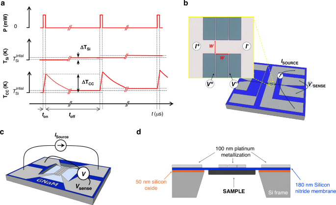
The microsecond-pulsed (μs-pulsed) nanocalorimetric method is a high-resolution thermal analysis technique derived from quasi-adiabatic scanning calorimetry. In this approach, the duration of the heating pulse is reduced to the microsecond range, producing a localized temperature increase of the calorimetric cell only a few Kelvin above the base temperature of the silicon frame. By applying current pulse trains with controlled duty cycles, ~50 µs ON and 100 ms OFF, the system remains near thermal equilibrium. Figure 1a shows a schematic of the train of pulses methodology. The duty cycle is chosen such that the calorimetric cell fully relaxes thermally between pulses, ensuring that each excitation starts from the same base temperature set by the substrate and sample holder, \({T}_{{\rm{Si}}}\). During each pulse, the applied current produces a rapid Joule heating of the suspended calorimetric cell, leading to a transient temperature rise \({\triangle T}_{{\rm{CC}}}\) of few K relative to \({T}_{{\rm{Si}}}\). Thus, \({T}_{{\rm{Si}}}\) represents the slowly varying base temperature of the substrate imposed by the cryostat temperature holder, while \({T}_{{\rm{CC}}}\) denotes the instantaneous temperature of the calorimetric cell induced by the microsecond pulse. During each local adiabatic heating pulse, after discarding the initial transient response, the calorimetric variables vary linearly, which allows considering time-averaged values for each variable within the ON-time window. Since the microsecond current pulse train is applied sequentially to the nanocalorimetric device, controlling the substrate temperature evolution enables additional signal averaging of the calorimetric magnitudes over repeated excitations at the same temperature, thereby enhancing sensitivity. This configuration allows heat capacity to be evaluated under quasi-static conditions, as in AC or relaxation calorimetry, while retaining the high heating rates and sensitivity characteristic of QAnC.
Fig. 1: Overview and working principle of the microsecond-pulsed nanocalorimeter.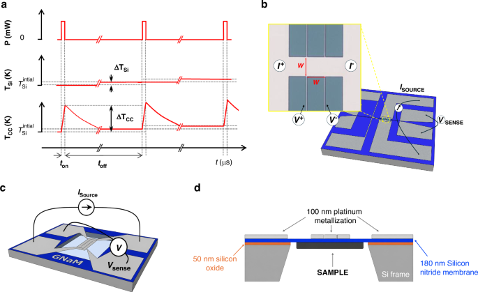
a Microsecond current pulses are applied to the nanocalorimetric device, with a duty cycle to ensure the cooling. \({T}_{{\rm{Si}}}\) denotes the base temperature of the substrate and sample holder, while \({T}_{{\rm{CC}}}\) corresponds to the transient temperature rise of the calorimetric cell induced by each pulse. b Strip-shaped heater/sensor with a square sensing area of side w (w = 30 µm, or 50 µm). Inset: magnified optical microscope image of 50 × 50 µm2 device. c Meander-shaped heater/sensor with a sensing area of 1 mm². d Cross-sectional schematic of the calorimeter, showing the silicon nitride membrane supporting the calorimetric cell at the center, including the metallic heater/sensor and the sample positioned underneath
Figure 1b–d presents different schematic views of the nanocalorimeters employed in this study. Each device consists of a freestanding silicon nitride (Si3N4) membrane, 180 nm thick, suspended over a silicon frame. Between the silicon nitride and the silicon there is a 50 nm thermally grown SiO₂ layer, which serves as an electrical insulation layer, preventing leakage currents and shunting. At the center of the membrane, a Ti/Pt bilayer (15/100 nm) defines the metallic element that functions both as a resistive heater and as a thermometer. Three distinct heater geometries were fabricated and tested: one meander-type design with a sensing area of 1 mm², and two strip-type designs with square sensing areas of 50 × 50 µm² and 30 × 30 µm², respectively. Samples, when present, are deposited on the backside of the silicon nitride membrane. A complete geometrical layout, dimensions and optical microscope images of the fabricated nanocalorimeters are explained in the Supplementary Information.
Principle of operation
Quantitative calorimetric measurements, irrespective of the specific architecture of the calorimetric cell, require the simultaneous determination of three key quantities: the time-dependent temperature of the cell, the electrical power input, and, under non-adiabatic conditions, the heat losses to the surroundings.
To operate the calorimeters, the local pulsed thermal excitation is achieved by injecting a controlled current \(I(t)\) through the metallic element. The resulting Joule heating induces a rapid temperature increase in the calorimetric cell, including the underlying dielectric membrane. The metallic element is designed in a four-probe configuration, allowing for localized measurement of the voltage drop \(V(t)\) at the calorimetric cell. The instantaneous power dissipated in the sensing area is calculated as \({P}_{{in}}\left(t\right)=V\left(t\right){\cdot I}\left(t\right)\), and the time-dependent resistance is given by \(R\left(t\right)=V\left(t\right)/I\left(t\right)\). These quantities, combined with a prior calibration of the resistance vs temperature relationship, enable accurate reconstruction of the temperature evolution \(T(R(t))\) and subsequent heat capacity analysis. After calibration, the platinum metallization exhibits an electrical conductivity of approximately 6.6 × 10⁶ S/m, with a temperature coefficient of resistance (TCR) of ≈0.0026 K⁻¹. At room temperature, the measured resistance is approximately ≈20 Ω for the meander-type design and ≈1.1 Ω for the strip-type sensors, with the sheet resistance being consistent across the different strip sizes. When injecting currents on the order of tens of milliamperes, the metallic element releases sufficient power to achieve heating rates on the order of 105 K/s. Operating at such a high heating rate the nanocalorimeter behaves quasi-adiabatic.
Under high vacuum conditions, heat losses from the calorimetric cell are limited to conduction through the membrane and thermal radiation and operating at such a high heating rate the nanocalorimeter behaves quasi-adiabatic. For instance, a meander-type calorimeter requires approximately 80 mW to reach a heating rate of 105 K/s, while the effective thermal conductance at room temperature is around 4 μW/K. Consequently, only after a temperature rise of ≈200 K, the power loss term \({P}_{{losses}}\) (4 μW/K × 200 K) reaches ≈1% of the input power \({P}_{{in}}\). Therefore, for short scans, heat losses can be neglected, while for longer scans, they must be considered. Details on how to account for these losses are provided in the Supplementary Information. In quasi-adiabatic conditions, nearly all the input power contributes to the internal energy of the calorimetric cell, and the apparent heat capacity \({{Cp}}_{\beta }^{{cc}}\left(t\right)\) measured approaches the real heat capacity of the calorimetric cell \({{Cp}}_{{real}}^{{cc}}\left(t\right)\), since \({{Cp}}_{\mathrm{real}}^{{cc}}\left(t\right)\) becomes negligible:
$${{Cp}}_{\beta }^{{cc}}\left(t\right)=\frac{{P}_{{in}}\left(t\right)}{\beta \left(t\right)}={{Cp}}_{{real}}^{{cc}}\left(t\right)+\frac{{P}_{{losses}}\left(t\right)}{\beta \left(t\right)}$$
(1)
where \(\beta \left(t\right)={dT}\left(t\right)/{dt}\) the measured heating rate.
In this framework, the measurement of a sample requires two consecutive measurements of the same calorimetric cell: first with the empty CC (denoted with superscript 0) and subsequently with the sample evaporated onto it (denoted with superscript 1).
$${{C}_{P}}^{{sample}}\,\left(T\right)\approx {{C}_{P}}_{\beta }^{{cc},1}\left(T\right)-{{C}_{P}}_{\beta }^{{cc},0}\left(T\right)$$
(2)
Analysis of the intrinsic noise in this measurement reveals that it is largely dominated by the numerical differentiation of digitized signals. Implementing true differential measurements significantly enhances the resolution.
The differential methodology can be implemented by connecting a pair of matched nanocalorimeters in series and performing the differentiation using a bridge of instrumentation amplifiers, as illustrated in Fig. 2. The differential voltage drop between the two calorimetric cells, defined as \(\triangle {\rm{V}}={{\rm{V}}}_{{\rm{S}}}-{{\rm{V}}}_{{\rm{R}}}\) where cell S hosts the sample (if any) and cell R serves as the reference, can be acquired with high amplification (typically ×10 to ×1000) using an instrumentation amplifier. The difference in apparent heat capacity between the two cells can then be recalculated by incorporating the differential voltage ∆V into the general expression (the complete derivation is provided in Supplementary Information)12,22:
$${{\mathbf{\Delta }}C}_{P}\left({T}_{S}(t)\right)=\frac{I\,\Delta V}{{\beta }_{S}}-\frac{{V}_{R}}{{\beta }_{S}\,{\beta }_{R}}\,\frac{{\left(d\Delta V/{dt}\right)}_{t}}{{\left(d{R}_{S}/d{T}_{S}\right)}_{t}}+\frac{{V}_{R}\,I}{{\beta }_{S}}\left[1-\frac{{\left(d{R}_{R}/d{T}_{R}\right)}_{t}}{{\left(d{R}_{S}/d{T}_{S}\right)}_{t}}\right]$$
(3)
Fig. 2: Electronic chain schematics.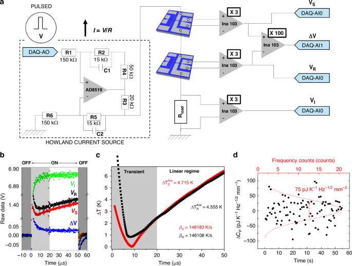
a (On the left) The ‘Howland’ Current Source based on a Op. Amplifier 8510, (On the right) an amplification bridge based on INA103, permit to measure the voltage dropped in the calorimetric devices, the differential signal and the current passing through a load resistor. b Raw data voltages acquired for a single pulse. c Temperature evolution of a couple of nanocalorimeters, showing transient zone and linear zone used to perform the evaluation of the variables. d Fluctuations around the mean value of the difference in heat capacity between twin nanocalorimeters (meander type) measured fixed temperature (150 K), as a function of time. The dispersion of the data determines the uncertainty of the measurement
Finally, in a complete experiment, the measurement of the sample’s heat capacity must account for the difference between the differential heat capacities of the calorimetric cells before and after sample deposition, in order to subtract any pre-existing offset (similarly to the procedure followed in non-differential measurements):
$${{C}_{P}}_{{diff}}^{{sample}}({T}_{S}(t))={\Delta{C}_{P}}^{1}\,-\,{\Delta{C}_{P}}^{0}$$
(4)
If large samples (compared to the calorimetric cell addenda) are loaded into the sample calorimetric cell, the resulting heating rates when the cell is loaded, \({\beta }_{S}^{01}\left(t\right)\) relative to the idle cell \({\beta }_{S}^{0}\left(t\right)\), may vary substantially, and the baseline subtraction may require an additional correction as proposed by Efremov et al22. Nevertheless, in the case of ultrathin samples such as those considered in this work, and given the very short duration of the temperature excursion, the accumulated temperature differences between the sample cell in the loaded and idle experiments are typically on the order of a few millikelvin. Combined with the fact that the variation in the cell’s heat capacity is also very small, the resulting beta correction falls well below the intrinsic noise level of the measurement and can therefore be neglected.
The analysis presented here, evaluates the thermodynamic variables of the calorimetric cell as a function of time during the local heating. As mentioned above in the microsecond-pulse regime, these variables exhibit linear behavior after discarding the initial transient response, which allows assigning averaged values for each pulse.
Instrumentation and electronics
The fast temporal dynamics of microsecond-pulsed nanocalorimetry necessitate a dedicated high-speed electronic setup. The system is built around a differential instrumentation amplifier bridge, where a pair of matched nanocalorimeters are connected in series with a precision load resistor (50 Ω). A schematic of the complete electronic chain is provided in Fig. 2a. Signal generation and acquisition are performed using a PXIe-6124 data acquisition card (National Instruments), which offers 16-bit resolution and supports simultaneous analog input/output at sampling rates up to 4 MS/s within a ± 10 V range. Synchronization and control of the pulse sequences are managed via LabVIEW software, which orchestrates the generation of current pulses by modulating the analogic output channel (DAQ-AO). The pulse parameters – including amplitude, pulse width (ton), and inter-pulse delay (toff) -are fully programmable, enabling precise control of the duty cycle.
To ensure stable and symmetric current delivery across varying load conditions, a Howland current source was implemented using an AD8519 operational amplifier (Fig. 2a). This voltage-to-current converter maintains a constant current through the bridge during microsecond-scale pulses and can deliver up to 67 mA in the regime used in our experiments. The Howland network was built using commercial precision 0603 SMD resistors with 1% tolerance, with the critical resistor ratios (R1/R6 and R2/R5) selected to ensure proper current-source operation. The output current is directly monitored via the voltage drop across a current-sense resistor (R3 = 20 Ω), allowing the pulse current and injected power to be reconstructed from measured quantities rather than inferred from nominal resistor values. This approach relaxes the requirements on absolute resistor matching while ensuring accurate current delivery under high slew-rate conditions. Small compensation capacitors (5 pF ± 0.25 pF, corresponding to ±5% tolerance) are included to improve stability and suppress high-frequency oscillations. The circuit design follows standard guidelines for Howland current sources, as described in Texas Instruments Application Note AN-1515 23.
Voltage signatures from the calorimetric bridge are pre-amplified using an INA103 instrumentation amplifier, chosen for its fast settling time (3 μs), ultra-low input noise (\(1{nV}/\sqrt{{Hz}}\) at 1 kHz), and high common-mode rejection ratio. The current delivered to each branch is monitored via the voltage drop across the load resistor (VI), enabling accurate reconstruction of both the instantaneous power input and the thermal response.
The initial voltage overshoot is associated with the circuit inductance responding to the high-frequency components of the current step, while the subsequent transient (~10 μs) is dominated by capacitive effects and the bandwidth-limited response of the Howland current source and instrumentation amplifiers. In optimized devices, the transient response remains below 10 μs. Considering the characteristic total resistance of the measuring circuit, the combined capacitance can be estimated at approximately 1 μF. A detailed discussion of the different impedance contributions and the device optimization required to minimize these effects is provided in the Supplementary Information.
Importantly, since the first 20 μs of the signal are discarded, the measurement is performed in the steady-state region where low-frequency components dominate and inductive and capacitive effects become negligible. This ensures that any phase difference between current and voltage does not affect the determination of thermometer resistance or power. Nevertheless, this constraint clearly imposes an upper limit on the achievable heating rates when the analyzed temperature window must remain restricted to only a few kelvin.
To conduct the experiments, the nanocalorimeters were mounted inside a custom-built liquid nitrogen immersion cryostat operating under high vacuum conditions (working pressures well below 10⁻7 mbar). The chamber was evacuated using a turbomolecular pump (Varian/Agilent Turbo-V 70) backed by a dry scroll pump (Agilent IDP-15). The devices were mechanically secured to an aluminum mount holder using clamps, and thermal contact was enhanced with either Apiezon N grease or silver paste. Given the high sensitivity of the measurements to base temperature fluctuations (δT₀), the temperature of the holder was actively controlled. For this purpose, the mount was equipped with a resistive heater powered by a Keithley 2400 source meter and monitored using a cryogenic Pt100 thermometer connected to a Keithley 2700 multimeter. A LabVIEW®-based control program implementing a PID algorithm was used to regulate the temperature setpoint. The use of high-precision source meters (6.5-digit resolution) enabled excellent thermal stability, achieving peak-to-peak temperature fluctuations below 1 mK. This setup allowed for both isothermal and temperature-ramp experiments across the full operational range of 80 to 450 K, a range limited not by the µs-PHnC technique but by the cryostat used and the low-temperature response of the Pt heater/sensor.
Figure 2b shows the raw voltage signals acquired during a single pulse experiment using a meander-type nanocalorimeter. The four recorded signals correspond to the sample (VS), reference (VR), current monitor (VI), and the amplified differential signal (100×ΔV). The acquisition is configured to capture data both before and after the pulse, enabling baseline offset correction for each channel, an essential step for accurate averaging across multiple pulses. The acquisition window includes the final part of the previous off-state (0–50 µs), the pulse-on interval (50–100 µs), and the beginning of the subsequent off-state (100–150 µs), as indicated in the figure. Only the pulse-on interval is used for calorimetric analysis. Figure 2c presents the corresponding temperature evolution of the sample and reference calorimeters. Two distinct regions are highlighted: an initial transient zone (shaded gray), dominated by the response time of the INA103 amplifier (≈3 μs), and a subsequent linear regime (white), where the temperature increases linearly with time. From this linear region, the average temperature rise after 50 μs was determined to be 4.715 K for the sample and 4.555 K for the reference. The corresponding heating rates, extracted from the slope of the linear fits, were 148183 K/s and 146108 K/s, respectively. To assess the noise density of the pulsed heating method, heat capacity was measured over 50-second intervals. Figure 2d displays the temporal fluctuations of the differential heat capacity signal (ΔCp) measured between two nominally identical nanocalorimeters at 150 K. Each black point corresponds to an individual measurement taken at a fixed acquisition rate. The dispersion of these values around zero is analyzed statistically, and the histogram of counts (top axis) is fitted by a Gaussian distribution (red curve). The standard deviation of this Gaussian represents the noise-equivalent fluctuation of ΔCp within the acquisition bandwidth. To express the resolution in a bandwidth-independent form, we normalize this standard deviation by the square root of the measurement bandwidth, yielding units of J K⁻¹ Hz⁻¹/² mm⁻². This allows comparing nanocalorimetry sensitivity across different acquisition times or instruments.
Using the experimentally determined noise-equivalent heat-capacity density of 75 pJ K⁻¹ Hz1/2 mm⁻², the corresponding noise floor for a reduced active area of 100 µm², representative of exfoliated two-dimensional flakes, is approximately 7.5 fJ K⁻¹ Hz1/2. For typical monolayer and few-layer 2D materials, whose expected heat capacities in this area range are on the order of 10–100 fJ K⁻¹ at room temperature, this translates into signal-to-noise ratios of order unity or higher with integration times of a few seconds. Longer integration times further improve the signal-to-noise ratio following the expected t1/2 scaling. Although direct calorimetric measurements on 2D materials are beyond the scope of the present work, this quantitative estimate suggests that the sensitivity achieved by µs-PHnC is sufficient for calorimetry at lateral dimensions relevant to exfoliated flakes.
Thermal modeling and scalability of the calorimetric cell
Ideally, the temperature across the calorimetric cell should remain homogeneous during calorimetric experiments. This condition is partially met in rapid heating experiments, where power is locally dissipated in the sensing area of the heater, and lateral heat diffusion induces transient temperature gradients. In calorimetric cells with a 1 mm² sensing area, this diffusion remains moderate even on millisecond timescales, allowing quasi-adiabatic operation. However, with the implementation of the microsecond-pulsed nanocalorimetry (µs-PHnC) method, the temperature profile improves substantially.
Finite element modeling of devices with silicon nitride membranes of 180 nm thick and 150 nm of Pt metalization (details provided in the Supplementary Information) reveals that under 50 µs pulses at heating rates of 100 kK/s, approximately two-thirds of the sensing area exhibit temperature differences below 2.5 K. In contrast, for 1 ms pulses, temperature variations can reach up to 20 K across two-thirds of the calorimetric cell. Although the thermal inhomogeneity inherent to the meander-type design can be mitigated by integrating additional metallic spreaders within the sensing area, this approach introduces a significant increase in heat capacity addenda, thereby compromising the overall sensitivity of the calorimetric cell 20.
Figure 3a, b display the simulated temperature maps and corresponding histograms for a meander-type calorimetric cell (1 mm²) at 50 µs and 1 ms, respectively.
Fig. 3: Thermal homogeneity and scalability of the calorimetric cell.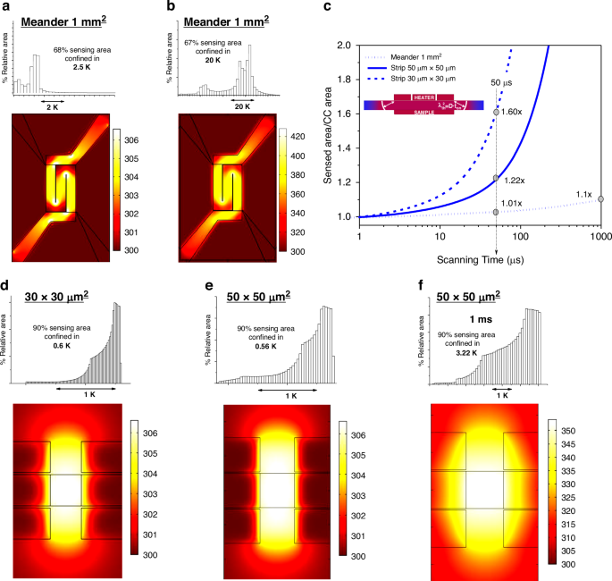
Temperature maps of a meander like calorimeter heated at 105K/s at times of a 50 μs and b 1 ms. The histograms show the 2D temperature dispersion in the calorimetric cell: showing that 2/3 of surface area is within 2.5 K after 50 µs from the start of the pulse while the temperature inhomogeneity degrades to 20 K after 1 ms. c Comparison of the sensed area normalized to the calorimetric cell (CC) area versus scanning time for three thermal sensing configurations: Meander (1 mm²), Strip (50 μm × 50 μm), and Strip (30 μm × 30 μm). d–f Show Simulated temperature maps for strip-type nanocalorimeters with sensing areas of 30 × 30 µm² and 50 × 50 µm². At 50 µs, 90% of the sensed area remains within a temperature range of 0.6 K and 0.56 K, respectively, indicating high thermal homogeneity. For the 50 × 50 µm² device at 1 ms, the temperature spread increases to 3.22 K, highlighting the impact of thermal diffusion over time on spatial uniformity
To assess how spatial temperature degradation under fast heating affects heat capacity measurements and limits calorimeter miniaturization, we used finite element modeling to show that the sensed heat capacity increases with thermal diffusion length, which scales with the square root of membrane diffusivity and time. The simulations reveal deviations in the measured heat capacity, and thus in the effective sensed area or heat capacity addenda, from the intrinsic values of the calorimetric cell. Figure 3c shows the normalized sensed area over time for different device geometries, based on comparisons between the heat capacity measured at a heating rate of 100 kK/s and the intrinsic heat capacity at the corresponding temperature, The inset schematically illustrates the thermal diffusion length λ, given by λ² = Dₜₕ·time, where Dₜₕ is the thermal diffusivity of the membrane. The analysis includes meander-type devices with 1 mm² sensing areas and strip-type nanocalorimeters with 50 × 50 µm² and 30 × 30 µm² sensing areas.
For meander-type devices with a ≈ 1 mm² sensing area, the sensed area increases by only ~1% after 50 µs (within the resolution limit) and reaches ≈10% after 1 ms. This moderate expansion follows a time dependence of t1/2 and remains manageable even at millisecond timescales. In quasi-adiabatic nanocalorimetry (QAnC), this effect can be mitigated by using differential measurements and by confining the sample to the original calorimetric cell with a shadow mask.
In contrast, for miniaturized strip-type devices with sensing areas of 50 × 50 µm² and 30 × 30 µm², the influence of thermal diffusion becomes significantly more pronounced. After 50 µs, the sensed area increases by approximately 22% and 60%, respectively. For these devices, the sensed area doubles the original calorimetric cell area after just 220 µs (50 × 50 µm²) and 80 µs (30 × 30 µm²), clearly demonstrating that long-duration pulses are unsuitable for small-scale designs. The rapid expansion of the sensed area severely limits sensitivity and imposes a fundamental constraint on the scalability of calorimetric cells and their applicability in QAnC.
The µs-PHnC method, operating in the tens of microseconds regime, effectively minimizes this diffusion-driven expansion. By maintaining a reduced sensed area, it also limits the heat capacity addenda, a key factor in enhancing sensitivity. This makes µs-PHnC particularly well-suited for high-resolution calorimetry in ultrasmall samples.
In addition to the broad variation in lateral device dimensions explored in this work, further miniaturization into the sub-micron regime introduces additional constraints that must be considered for future implementations. At these length scales, the thermal diffusion length during a 50 µs pulse becomes comparable to the footprint of the device, making thermal uniformity increasingly sensitive to both the scan speed and the exact geometry of the heater–thermometer strip. Accurate sample delineation also becomes non-trivial at sub-micron scales: lithographically defined shadow masks or well-aligned deposition windows are required to prevent overspread of material beyond the active region, which would otherwise dominate the heat-capacity signal.
Figure 3d–f)presents simulated temperature profiles for strip-type devices with sensing areas of 30 × 30 µm² and 50 × 50 µm². At 50 µs, the heated region closely matches the heater footprint, which represents the ideal scenario. However, a narrow region surrounding the heater also becomes heated due to thermal diffusion, extending a few micrometers beyond the active area. This effect is more noticeable in the smaller device and becomes increasingly significant at longer pulse durations, as shown in Fig. 3c.
The improvement in temperature homogeneity is evident. For the 50 × 50 µm² calorimeter, 90 percent of the sensed area falls within a temperature range of 0.56 K at 50 μs, as shown in the histogram. As expected, increasing the pulse duration or reducing the device size leads to greater temperature dispersion. For example, at 50 μs, the 30 × 30 µm² device shows a temperature spread of 0.6 K, while the 50 × 50 µm² device reaches 3.22 kelvin at durations of 1 ms. These results highlight the trade-off between temporal resolution and spatial uniformity in miniaturized calorimetric designs.