
Lidar and time-offlight (ToF) systems depend on fast, stable and repeatable laser pulses, write Laephar Castro and Anant Sinha.
The growing adoption of autonomous vehicles, industrial automation and advanced robotics is increasing demand for reliable 3D ranging and sensing. Lidar and time-offlight (ToF) systems rely on precisely controlled laser pulses to measure distance and spatial information. Meeting these requirements demands laser drivers that deliver high peak current and maintain pulse-to-pulse stability across temperature and ageing. Traditional discrete topologies that use gate drivers, external field effect transistors and current-sensing elements can meet specific design requirements; however, they often introduce trade-offs in terms of layout complexity, calibration effort and thermal performance.
Laser drivers directly influence the timing information that lidar and ToF systems use to calculate distance. Consider a simple timing variation budget comprising of several sources, where there are three contributors:
1 Rise and fall time (tr/f): how quickly the pulse moves through the detection threshold.
2 Propagation delay (tpd): how long it takes from the trigger to actual light emission.
3 Pulse-to-pulse variation (tpp): how much the timing or amplitude drifts from pulse to pulse.
Lidar and ToF systems measure the distance by calculating the round-trip time for a laser pulse to travel to a target and return to a receiver. The ability to distinguish small distance changes depends on how quickly the pulse edges transition between no light and full light. Faster rise and fall times reduce distance uncertainty and give the receiver a clearer reference point. In high-resolution systems rise and fall times typically range from 1ns to 5ns.
When a pulse edge is slow the system cannot determine the exact moment the signal crosses the receiver detection threshold. A tr/f equal to a 1ns edge therefore introduces about 150mm of distance uncertainty, approximated by Equation 1:
ctr/f
∆ D = _____2 (1)
where ΔD is the delta distance and c ≈ 3×10⁸m/s.
This uncertainty increases with slower pulse edges, which parasitics such as package and printed circuit board inductance can limit, along with the capacitance of the laser diode and driver output.
If the propagation delay changes with temperature, supply voltage or component tolerances, it shifts the timing reference used for distance calculations and can disrupt synchronisation between channels. In direct ToF applications, a 100ps variation in tpd corresponds to roughly 30mm of distance error, based on the ToF relationship shown in Equation 2:
D = c×t (2)
where c ≈ 3×10⁸m/s, D is the distance and t is the time.
Any excess delay directly translates into ranging error.
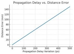 Figure 1: Propagation delay vs. distance error (estimated)
It is possible to calibrate fixed delays during system alignment, but variable delays such as self-heating introduce measurement-to-measurement uncertainty that is not easily correctable.
Even a fast, narrow laser pulse must remain consistent from one pulse to the next. Variations in peak current translate directly into changes in optical power, degrading measurement accuracy and system reliability.
Temperature shifts, supply fluctuations and device ageing are common sources of this drift.
From a system perspective, the receiver relies on the returned optical signal to determine distance. Differences in pulse strength can therefore be misinterpreted as range variation, particularly at long distances where return signals approach the detection threshold. In threshold-based ranging systems, a 1% change in peak current produces roughly a 1% change in optical power, which can introduce distance errors on the order of tens of centimetres. As shown in Figure 2, even modest amplitude variations of ±2% to ±5% can alter the pulse envelope and optical energy delivered per pulse, reducing ranging accuracy and repeatability over time. High-performance designs therefore tightly control the drive current, keeping tpp variation within a few percent across all operating conditions.
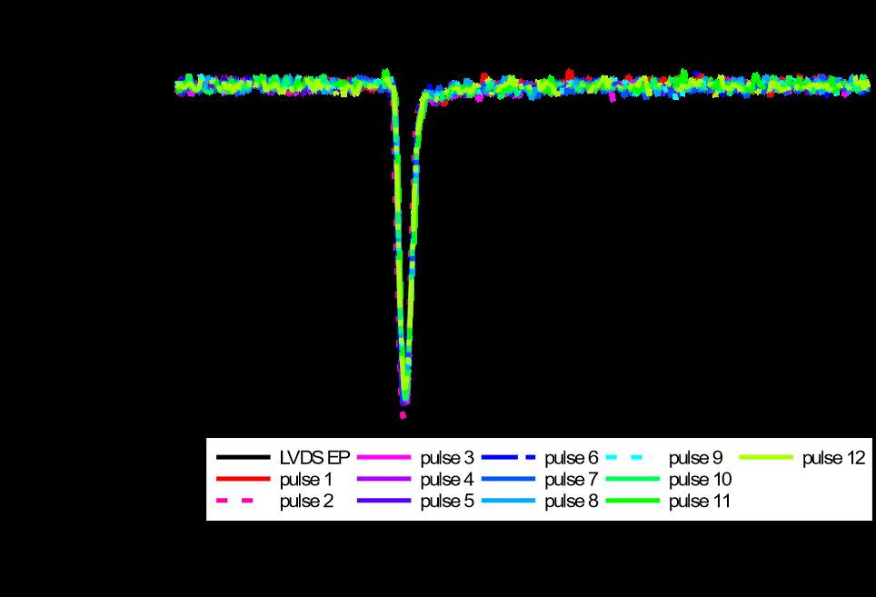
Figure 2: Pulse-to-pulse amplitude for 12 pulse, 1.5A current
Rdamp =1Ω and 2 snubber pair of 5Ω resistor and 330pF cap, AVDD = PVDD = VLD = 5V
With the system-level timing constraints defined, the next step is translating them into a practical laser driver implementation.
Generating accurate laser pulses requires the driver to deliver high peak currents with fast edges, predictable delay and repeatable pulse amplitude. TI’s LMH13000 high-speed laser driver generates pulses by converting the input voltage at the VSET pin into a precisely regulated sink current at IOUT, as described by Equation 3. A digital-to-analogue converter or reference source sets VSET, while the device’s internal current mirror and control circuitry regulate the current through the laser diode, as shown in Figure 3. Careful selection of VSET, RSET and the laser anode bias voltage allows designers to tune the pulse amplitude, timing and overall pulse stability.
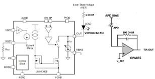
Figure 3: Circuit schematics transmit path block diagram with a diode and the LMH13000
Here are the design steps for setting pulse current and speed.
1. Define the target output current (IOUT). Begin with the optical power that the laser diode requires. Equation 3 expresses the peak output current, set by the laser’s slope efficiency:
POPT_____ (3)
IOUT = η
where POPT is the desired optical output power and η is the laser’s slope efficiency (watts per ampere). For example, if POPT = 1W and η = 0.5W/A, then IOUT = 2A.
Because the LMH13000 supports pulsed currents up to 5A, the selected laser diode must achieve the target optical power at or below this limit. Accurately setting IOUT minimises tpp and reduces amplitude-driven timing errors.
2. Select RSET and VSET. The LMH13000 sets the output current using the ratio of VSET to RSET, scaled by an internal gain factor k (Equation 4):
VSET_____ (4)
IOUT = RSET×k
In high-current mode (MODE = 1), k ≈ 50k. For example, with RSET = 20kΩ and VSET = 0.8V:
IOUT = 200.8k×50k ≈ 2.0A
It is possible to make fine adjustments by trimming VSET with a DAC. This approach minimises sensitivity to temperature and supply variations, helping keep tpp small within the timing budget.
3. Set the VLD. VLD must be high enough to support the laser forward voltage and dynamic voltage required during fast current transitions. The LMH13000 datasheet provides Equation 5 as a sizing guideline:
VLD = VOUT MIN+VFL×dtdI+IOUT×RLASER+RDAMP (5) where:
VIOUT is the minimum compliance voltage at IOUT
VF is the forward voltage of the laser at IOUT
L is the total loop inductance (package and PCB)
dI/dt is the current slew rate (amperes per second) from rise and fall requirements
RLASER is the dynamic resistance of the laser diode
RDAMP is the external resistance of the laser diode.
For example, with:
VIOUT(MIN) = 6V
VF = 2V
L = 3nH
dtdI = 12nsA = 2×10⁹A/s
RLASER = 0.3Ω
RDAMP = 1Ω
VLD ≈ 6+2+3×10⁻⁹ 2×10⁹+2 0.3+1.0 ≈ 16.6V
A starting value of 17V is therefore appropriate. Increasing VLD improves the edge speed but can increase overshoot, thus requiring careful tuning. Proper VLD selection ensures fast transitions while limiting overshoot, directly reducing the rise and fall time (tr/f) contribution to the overall total timing variation (ttotal) budget.
4. Optimise rise and fall times and damping. Both driver capability and circuit parasitics set the rise and fall times. Fast current pulse transitions can excite ringing in the laser and PCB loop, causing overshoot and unstable optical pulses. Designers commonly address this by adding a damping resistor and snubber network at the IOUT node. Together, the resistor and snubber suppress parasitic ringing, preserve fast edges and prevent tr/f from unnecessarily increasing the total.
Select snubber capacitors based on the output capacitance of the driver, calculated using Equation 6:
CSNUB ≈ 5×CIOUT (6)
where CIOUT is the effective capacitance at the IOUT pin. If CIOUT = 40pF, then CSNUB ≈ 200pf.
Adding a small damping resistor in series with the laser and snubber network suppresses unwanted oscillations. As shown in Figure 4, typical values for RDAMP and RSNUB are in the 5Ω to 10Ω range, with the snubber capacitor sized to the output node capacitance. Select CSNUB for the worst case (highest) CIOUT, trimming during validation to balance overshoot and edge speed. As illustrated in Figure 5, this approach reduces ringing from fast transitions and PCB parasitics, while preserving the sub-nanosecond tr/f required for precise pulse control.
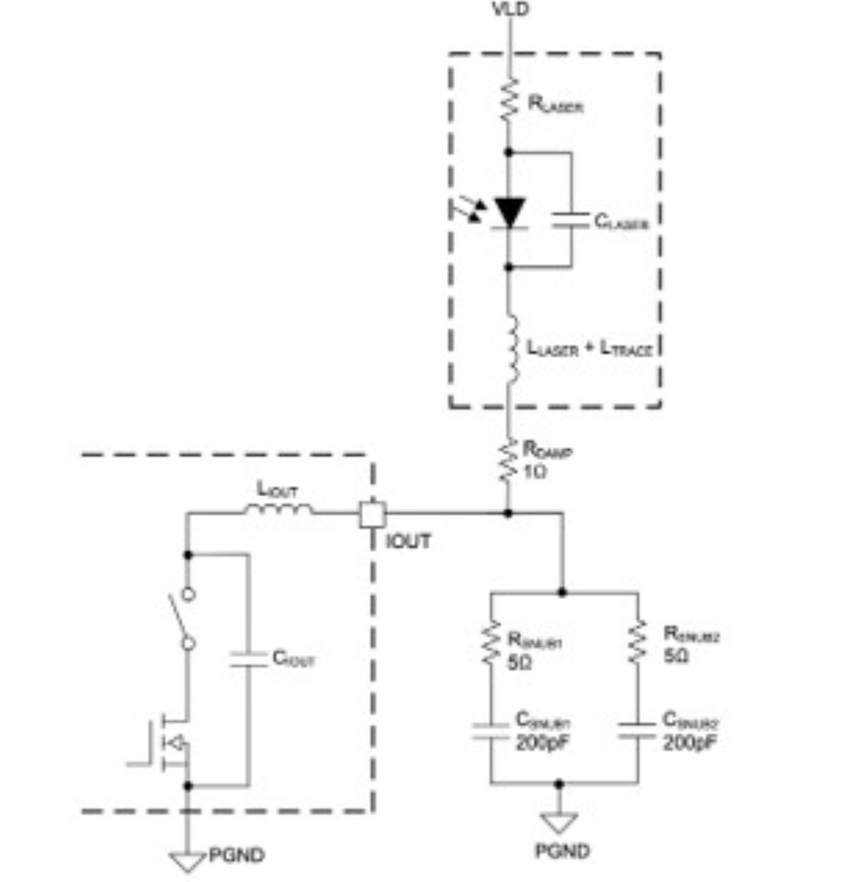
Figure 4. Damping resistor and snubber network circuit
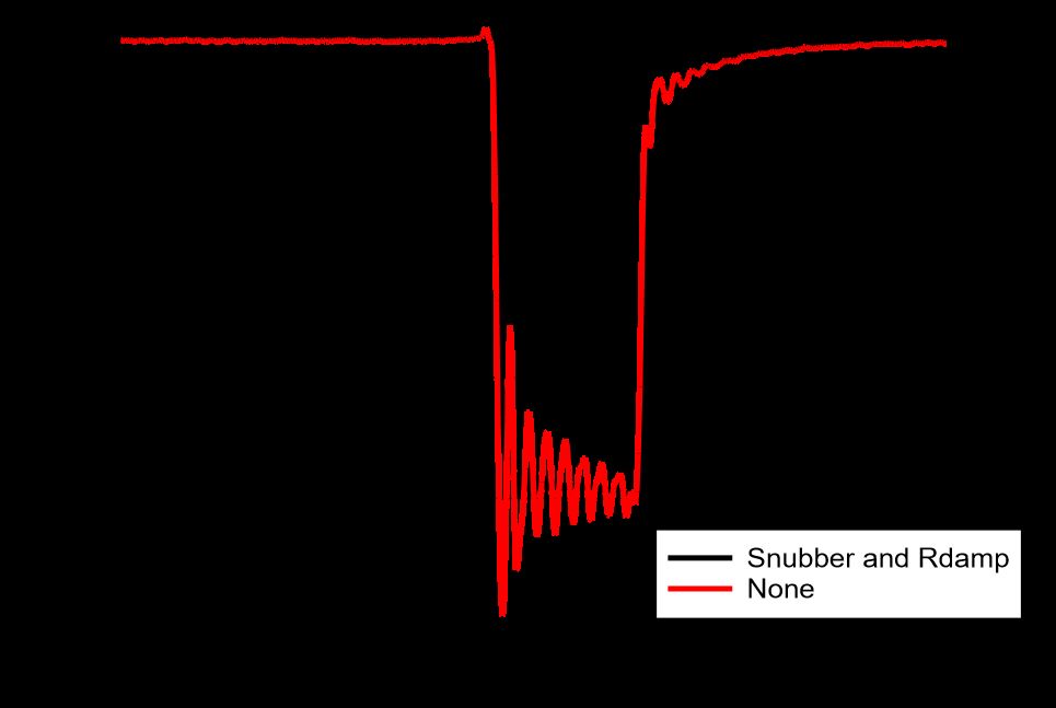
Figure 5. The LMH13000 pulse with and without a snubber circuit or RDAMP
5. Control the propagation delay. Unlike rise and fall times, propagation delay is not defined by a formula, but depends on these layout and interface practices:
Input routing. Use differential routing for EP pin and EN pin with 100Ω termination, or route a single-ended input with controlled impedance and proper termination at the LMH13000 input.
Output loop. Keep the high-current IOUT loop short and tightly coupled to PGND to minimise inductive delay and ringing.
System calibration. Account for any residual system delay by including the driver-laser path in the ToF measurement budget.
Minimising the trace inductance and ensuring consistent input termination reduces variation in tpd, keeping this contribution small and predictable. For applications that require higher accuracy or where temperature-based calibration is not practical, The LMH13000 datasheet presents a technique for high-accuracy start-pulse generation by directly monitoring the laser stage.
As shown in Figure 6, minimising the trace inductance and ensuring consistent input termination reduces variation in tpd, keeping this contribution small and predictable. For applications that require higher accuracy or where temperature-based calibration is not practical.
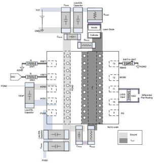 Figure 6: Layout example of the LMH13000 in the surface-mount device package
Lidar and ToF systems typically operate in pulsed mode, generating high-current bursts separated by long off-times. In this mode, the current waveform must settle quickly and reach the same peak value on every pulse. A common approach is to pre-bias the laser anode through VLD and use low-voltage differential signalling (LVDS) inputs (EP, EN) to gate the pulses. This enables VSET pin to set the amplitude while the LVDS inputs independently control the timing.
With RDAMP = 2.6Ω, VLD = 12V and IOUT = 400mA (laser diode: Osram’s PLT5 518FB_P), Figure 7 shows the lab result with a laser diode. In the figure, blue is enable, yellow is the start pulse and orange is VANODE. Decoupling amplitude and timing minimises pulse-to-pulse drift and preserves fast edges, improving both amplitude stability (tpp) and edge consistency (tr/f), further lowering the total.
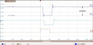
Figure 7: Precise pulse control in pulsed mode
Testing the LMH13000 under the lidar transmitter conditions shown in the table below validates the design principles.
Design parameters
Diode
V105Q121A-940
Analogue VDD and power VDD
5V
Mode
1
Pulse current
2A peak
Pulse width
0.6ns, 0.7ns
RSET
20kΩ
VSET
0.5V (set by the DAC)
VLD
4.5V, 5V, 6.5V
Design parameters
Damping network
RDAMP = 1Ω
RSNUB = N/A
CSNUB = N/A (no snubber)
Table: Design parameters for LMH13000 pulse driver example
Figure 3 shows the test setup, which illustrates the circuit schematic used to bias the laser and configure the LMH13000.
Figure 8 shows the optical response of the LMH13000 at different VLD bias voltages during pulsed operation. The transient waveforms illustrate how VLD directly affects rise times, overshoot and steady-state current regulation. A lower VLD results in slower edge transitions, while a higher VLD improves speed but may increase overshoot. Selecting the appropriate VLD, therefore, balances tr/f against pulse stability to minimise its contribution to the overall variation budget.
This design demonstrates how careful biasing and damping produce fast, stable optical pulses with minimal overshoot and repeatable performance. Based on the variation budget, this design achieves tr/f <1ns, tpd variation <50ps, and tpp <2%. Together, these results yield a total well below 1ns, enabling millimetre-level range precision.
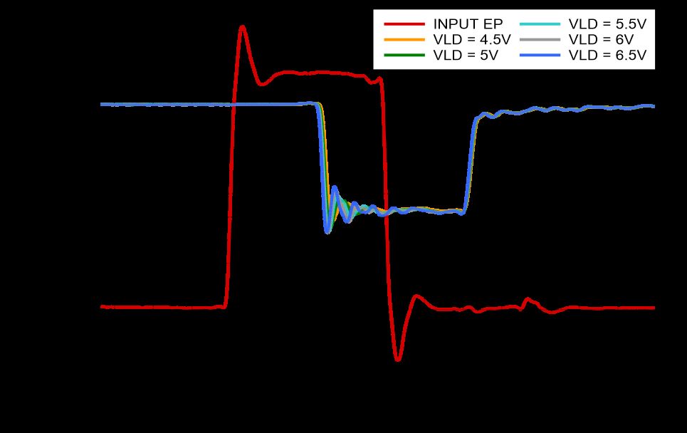
Figure 8: Optical response at a 4.5, 5, 5.5, 6 and 6.5 VLD bias voltage
Precise laser pulse control requires balancing edge speed, timing accuracy, stability and optical power consistency. Integrating high-speed current drive and regulation into a compact solution reduces design complexity while improving repeatability and performance. When combined with simple feedback and temperature monitoring techniques, this laser driver provides a reliable platform for both continuous and pulsed laser operation, enabling reliable and accurate performance in demanding lidar, ToF and industrial optical sensing applications.
Leaphar Castro is a product marketing engineer at Texas Instruments and Anant Sinha is an applications engineer at Texas Instruments.
See: World’s first net 400 Gps optical link employing an APD receiver