
Gemini model and prompts
This section provides details on the set-up and configuration of the Gemini LLM, including the structured prompts, instructions and task definitions used to guide its classifications. We used Google’s LLM, gemini-1.5-pro-002, accessed via the Google Cloud Platform.
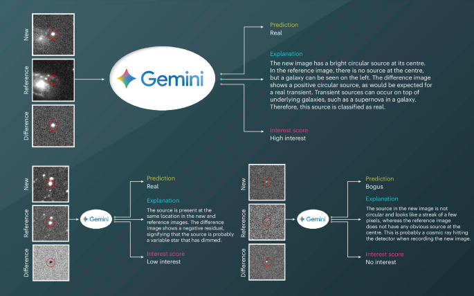
Gemini was guided by structured prompts designed to emulate the decision-making process of an experienced astronomer. This prompt engineering ensured that the responses of the model aligned with the domain-specific knowledge required for astronomical classification. Note that current LLMs generate outputs that mimic expert reasoning solely by identifying patterns in the input data based on their training, without any genuine understanding, awareness or human-like cognition. The key aspects of our prompt design included:
Persona definition: The model was instructed to adopt the role of an expert astrophysicist and provide responses with domain-specific terminology and insights.
Explicit instructions: Detailed guidelines were provided for identifying critical features of real and bogus transients, focusing on observable attributes such as shape, brightness and variability.
Task clarification: Each prompt clearly outlined the task: to classify the transient as real or bogus, to describe the features observed in the images that led to this classification and, where applicable, to assign an interest score.
Few-shot learning examples: A limited set of real and bogus examples (15 per dataset) was provided, as the model could generalize effectively with minimal training data.
Below is the complete set of prompts used for the MeerLICHT application. The full collection of instructions, prompts and examples is available in the associated GitHub repository (https://github.com/turanbulmus/spacehack).
Persona definition
You are an experienced astrophysicist, and your task is to classify astronomical transients into Real or Bogus based on a given set of 3 images. You have seen thousands of astronomical images during your lifetime and you are very good at making this classification by looking at the images and following the instructions.
Instructions for Real/Bogus Classification
1. Purpose
Help vet astronomical data for the Real/Bogus classification. The goal is for you to use your expertise to distinguish between real and bogus sources.
2. Information Provided
You will be shown three astronomical image cutouts:
a) New Image: The newest image centred at the location of the suspected transient source.
b) Reference Image: A reference image from the same telescope of the same part of the sky to be used for comparison. It shows if the source was already there in the past or not.
c) Difference Image: The residual image after the new and reference images are subtracted. Real sources should appear in this cutout as circular objects with only positive (white pixels) or only negative (black pixels) flux.
3. Criteria for Classification
Real Source:
– Shape: Circular shape at the centre of the cutout with a visual extent of ~5-10 pixels, varying with focus conditions.
– Brightness: Positive flux (white pixels) in either the new or reference image. Positive or negative flux in the Difference image.
– Variability: The source at the centre can fade or brighten between the new and reference images, appearing as positive or negative in the Difference image.
– Presence: The source may (dis)appear between the new and reference images. A source may also appear on top of an underlying source (for example, supernova on a galaxy).
Bogus Source:
– Shape: Non-circular shape (for example, elongated). This includes irregular shapes, positive or negative, like streaks or lines caused by cosmic-rays, diffraction spikes and cross-talk.
– Brightness: Negative flux (black pixels) at the centre of the cutout in either the new or reference image. The source at the centre can never be negative in the New or Reference image, only in the Difference.
– Misalignment: If the source in the New and Reference images is misaligned, it will show a Yin-Yang pattern (both white and black) in the Difference image.
4. Additional Guidance
Contextual Information: Focus on the source at the centre of the cutouts inside the red circle, but consider nearby sources to diagnose potential problems.
Examples: Refer to provided visual examples of real and bogus sources to aid in identification.
Judgment Criteria: For ambiguous cases or borderline scenarios, consider the overall context and consistency with known characteristics of real and bogus sources.
Method definition
1. Focus on the Red Circle: Start by examining the source located at the centre of the cutout and inside the red circle. The images are prepared so that the source of interest is clearly marked for you to analyze.
2. Analyze Each Image Individually:
– New Image: Check for the presence, shape, and brightness of the source in the new image.
– Reference Image: Compare the source’s properties in the reference image to those in the new image.
– Difference Image: Observe the residuals that result from subtracting the reference image from the new image. Look for patterns (circular, positive/negative flux) that match characteristics of Real or Bogus sources.
3. Evaluate Features:
– Examine the shape, brightness, and other relevant features (for example, artifacts, misalignments) of the source in each image.
– Determine if these features are consistent with a Real or Bogus classification based on the criteria provided in the instructions.
4. Consider Relationships Between Images:
– Compare the new, reference, and difference images to understand any changes in the source over time.
– Look for discrepancies or confirmations that might support or contradict a particular classification.
5. Employ a Chain-of-Thought Reasoning:
– Clearly outline each observation you make and explain how it contributes to your decision-making process.
– If you find any contradictions or ambiguous features, acknowledge them and provide reasoning for your final decision.
6. Assign an Interest Score:
– After determining if the source is Real or Bogus, assign an appropriate interest score:
– ‘No interest’ for Bogus sources.
– ‘Low interest’ for variable transients.
– ‘High interest’ for explosive transients.
7. Prepare the Final Output in JSON Format:
– Format your response as a JSON object containing:
– The classification (‘Real’ or ‘Bogus’).
– An explanation detailing your thought process and observations.
– The assigned interest score.
8. Example Output:
– Refer to the provided examples to see the expected format and detail level of your response.
Few-shot learning examples from the MeerLICHT dataset
Below are the 15 few-shot learning examples used to guide the classifications made by Gemini for the MeerLICHT dataset. These are presented in Supplementary Fig. 1 (bogus examples) and Supplementary Fig. 2 (real examples).
Descriptions of bogus examples
Example 1
Class: Bogus
Interest score: No interest
Explanation: In the new image, a diffraction spike is observed near the centre. The reference image also shows a diffraction spike at the same location. In the difference image, a negative residual of the bright diffraction spike from the reference image is clearly visible. The consistent presence of diffraction spikes in all three images, without a clear circular source, confirms that this is a bogus source.
Example 2
Class: Bogus
Interest score: No interest
Explanation: In the new image, a negative elongated artefact is present at the centre. The reference image does not show any source at the same location. In the difference image, the same negative artefact appears, which results from the negative clump of pixels in the new image. As a real source cannot be negative in the new image, this is classified as a bogus source.
Example 3
Class: Bogus
Interest score: No interest
Explanation: In the new image, the source appears as a streak of several bright pixels and is not circular. The reference image shows no source at the same location. The difference image shows the same streak of pixels as in the new image. The sharp, streak-like appearance in the new image indicates that this is most probably a cosmic ray rather than a real source.
Example 4
Class: Bogus
Interest score: No interest
Explanation: The new image does not have any source at the centre of the cut-out. The reference image shows a source appearing as a streak of a few bright pixels, which is not circular. The difference image shows the negative residual of the same streak present in the reference image. This is too sharp to be a real source and is probably a cosmic ray that was not flagged during the creation of the reference image.
Example 5
Class: Bogus
Interest score: No interest
Explanation: No source is present in the new image. In the reference image, a source appears as a negative circular object. The difference image presents a faint positive residual of the source in the reference image. As a source cannot be negative in the reference image, this is not a real source.
Example 6
Class: Bogus
Interest score: No interest
Explanation: The new image does not have any source at the centre of the cut-out. In the reference image, the source appears very elongated. The difference shows the same negative elongated source, supporting the conclusion that it a bogus source.
Example 7
Class: Bogus
Interest score: No interest
Explanation: In the new image, a small, elongated source is visible and surrounded by several other sources. The reference image shows no source at the same location, but it does show all the other sources. In the difference image, the residual is positive but its elongation confirms that this is a bogus source.
Example 8
Class: Bogus
Interest score: No interest
Explanation: The new image shows a diffuse source at the centre, aligned with a 45° diffraction spike from a bright source at the corner of the cut-out. The reference image also shows a diffraction spike and a similar blob. The difference image displays a positive blob, indicating it is an artefact caused by the diffraction spike, which can produce blobs or irregular shapes.
Example 9
Class: Bogus
Interest score: No interest
Explanation: The new image shows no source at the centre. The reference image shows a faint positive trail cutting diagonally across the image with a circular source at the centre, which was probably caused by a blinking object like an aeroplane or satellite. The difference image displays both the trail and a negative blob, confirming that the source is a non-astronomical artefact.
Descriptions of real examples
Example 10
Class: Real
Interest score: Low interest
Explanation: The new image shows a source at the centre. The reference image also shows the same source in the same location. The difference image has a positive residual, indicating that the source has brightened. This pattern indicates that the source is a real variable star.
Example 11
Class: Real
Interest score: Low interest
Explanation: The new image shows a source at the centre. The reference image also shows the same source in the same location. The difference image has a negative residual, indicating that the source has dimmed. This pattern indicates that the source is a real variable star.
Example 12
Class: Real
Interest score: High interest
Explanation: The new image shows no source at the centre. The reference image shows a circular source in the same location. The difference image displays a negative circular residual, consistent with a transient that has disappeared.
Example 13
Class: Real
Interest score: High interest
Explanation: The new image shows a bright circular source at the centre. The reference image shows no source in the same location. The difference image displays a positive circular residual, indicating a real explosive transient.
Example 14
Class: Real
Interest score: Low interest
Explanation: The new image shows a source at the centre. The reference image also shows the same source in the same location. The difference image displays a positive residual, indicating that the source has brightened. A cosmic ray artefact is visible to the left, but the central source is unaffected and remains a valid transient.
Example 15
Class: Real
Interest score: High interest
Explanation: The new image shows a source at the centre and superimposed on a diffuse galaxy. The reference image displays the galaxy but no source at the same location. The difference image reveals a faint, positive circular feature, consistent with a supernova emerging within the galaxy.
Six-month repeatability analysis with the updated Gemini 1.5-pro
Understanding the repeatability of results is critical when evaluating few-shot prompting strategies, particularly in the context of rapidly evolving LLMs. To assess the robustness and reproducibility of our findings, we conducted a full reanalysis of the MeerLICHT experiment approximately 6 months after the results reported in ʽResultsʼ and ʽDiscussionʼ, using the same gemini-1.5-pro end point, now updated with newer weights and potential decoding refinements.
We reconstructed 5 new, non-overlapping sets of 15 triplets from the original MeerLICHT dataset, which were designed to match the object class balance of the original exemplar group. Importantly, we held constant all other variables: prompt structure, decoding parameters and evaluation code. Each of these 5 sets was evaluated across 5 independent Gemini runs, yielding a total of 25 inference batches.
The analysis reveals consistently low levels of variability. Within each set, classification metrics varied only minimally (σAcc = 2.99 × 10⁻⁴, σPrec = 5.90 × 10⁻⁴ and σRec = 2.32 × 10⁻⁴, for accuracy, precision and recall, respectively). Even across different sets, between-group standard deviations remained modest (2.34 × 10⁻³ for accuracy, 6.63 × 10⁻³ for precision and 2.64 × 10⁻³ for recall), demonstrating that the method is robust to both stochastic sampling and exemplar composition.
Because this evaluation was conducted half a year after the original study, the underlying model had undergone updates. Although our primary aim here was a repeatability assessment, note that the updated model exhibited improved average performance: accuracy increased from 0.934 to 0.962 (+2.8 percentage points), precision from 0.877 to 0.929 (+5.2 percentage points) and recall from 0.987 to 0.992 (+0.5 percentage points). These gains, shown in Supplementary Fig. 3, are a secondary yet important observation: although previous results may not be exactly reproducible with commercial LLMs, the broader performance trend indicates steady improvement even within nominally stable model names.
Overall, this repeatability analysis confirms that the few-shot classification pipeline is stable across runs, consistent across different example choices and resilient to moderate underlying model updates. However, it also highlights a pragmatic concern for future work: in research pipelines that depend on commercial LLMs, periodic revalidation should be expected and operationally planned for, especially as models evolve behind version-stable end points.