
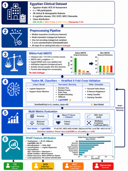
Figure 1 maps the full pipeline. Data came from 140 Egyptian patients assessed with the validated Egyptian Arabic ACE-III, producing 28 clinical and demographic features labelled across four cognitive classes: CN, SCD, MCI, and Dementia. Those raw records passed through a preprocessing sequence of median and mode imputation, one-hot encoding, and z-score standardisation fitted on the full dataset prior to cross-validation (the dataset has no missing values, so imputation has no practical effect regardless of fit scope). SMOTE then corrected the 10:1 class imbalance that is typical of Egyptian outpatient cognitive screening cohorts, applied inside each training fold only so synthetic samples never touched the validation data. Twelve classifiers drawn from five algorithm families (linear, kernel-based, tree-based, gradient-boosted, and meta-ensemble) were trained and evaluated under stratified five-fold cross-validation, each model seeing identical experimental conditions with no hyperparameter advantage given to any. LightGBM came out on top across the metrics that matter most: macro F1-score 0.723, ROC-AUC 0.944, balanced accuracy 0.716, Cohen’s κ 0.729, and MCC 0.733, though a paired t-test found this advantage statistically significant against only one of the eleven remaining classifiers at this sample size. Finally, SHAP explanations were computed using the estimator appropriate to each model type (TreeExplainer, KernelExplainer, LinearExplainer), consistently identifying age, educational attainment, and depression as the three dominant predictors. A feedback arrow from the evaluation stage back to classifier training represents the retraining loop available for prospective clinical deployment; each stage is described in detail in the upcoming subsections.
Fig. 1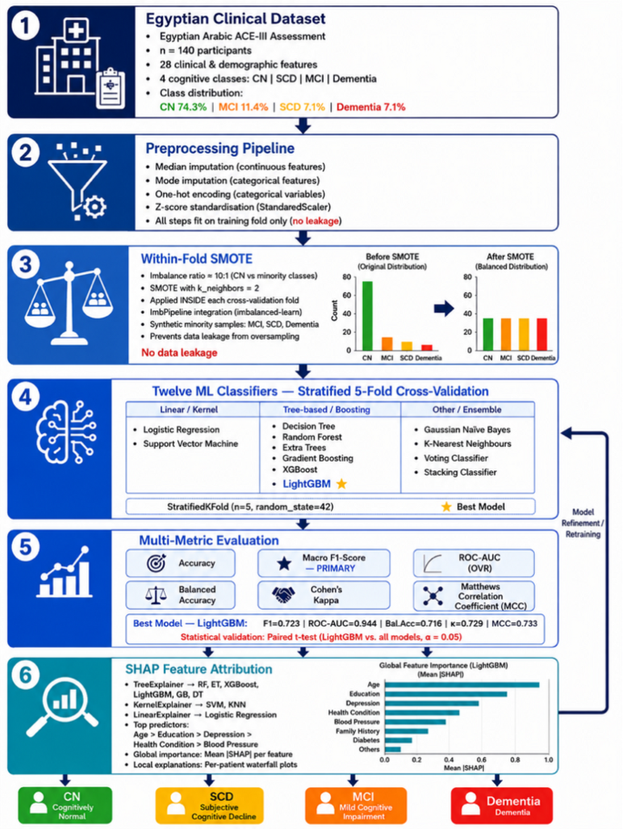
Proposed research framework for multiclass cognitive decline classification using the Egyptian Arabic ACE-III.
Study design and dataset
All data came from Egyptian patients assessed with the validated Egyptian Arabic ACE-III33,35 in a single Egyptian clinical setting (Table 2). After preprocessing, the dataset comprised 140 participants and 28 features. The class distribution was heavily skewed: 74.3% cognitively normal (Fig. 2), leaving MCI, SCD, and Dementia each below 12%. That 10:1 imbalance is the central challenge the pipeline was built to handle. The sample size (n = 140) reflects all patients meeting inclusion criteria who completed the Egyptian Arabic ACE-III assessment at the study site during the recruitment period, rather than a target derived from a priori power analysis. As this was a retrospective, single-centre clinical dataset rather than a prospectively designed and powered study, no formal priori power calculation was performed.
Feature set
The 28 features cover demographics (age, sex, marital status, education, occupation) and clinical risk factors: depression scores, blood pressure, diabetes, family history of MCI or Alzheimer’s disease, and composite health indices all derived from the Egyptian Arabic ACE-III encounter. Educational attainment was encoded using an ordinal scale aligned with the Egyptian national education system, reflecting the substantial variation in schooling access across Egyptian generations and regions. The Pearson correlation matrix (Fig. 3) shows low inter-feature correlation: each variable captures a distinct clinical dimension.
Notably, the underlying dataset also includes itemized ACE-III scores for all five cognitive domains (Attention/Orientation, Memory, Fluency [recorded as two verbal-fluency subtests], Language, Visuospatial) alongside the ACE-III total score. None of these seven scores were included among the 28 classification features: each was one of the factors clinicians used, alongside clinical history and other findings, to assign a patient’s diagnostic label, so including any of them as predictors would create circularity between predictor and target. The resulting feature set — demographics and clinical/vascular risk factors — is not intended to reproduce the ACE-III’s own cognitive measurements, but to test how much of a patient’s eventual diagnostic category can be predicted from information already available in routine clinical care, independent of administering and scoring the ACE-III itself. This frames the model as a pre-screening or triage aid rather than a substitute for the instrument; whether adding these itemized subdomain scores as predictors would improve classification accuracy is a direct empirical question we leave to future work (Sect. 5.7).
Table 2 Dataset features: demographic, clinical, and cognitive characteristics of the study sample (n = 140).Fig. 2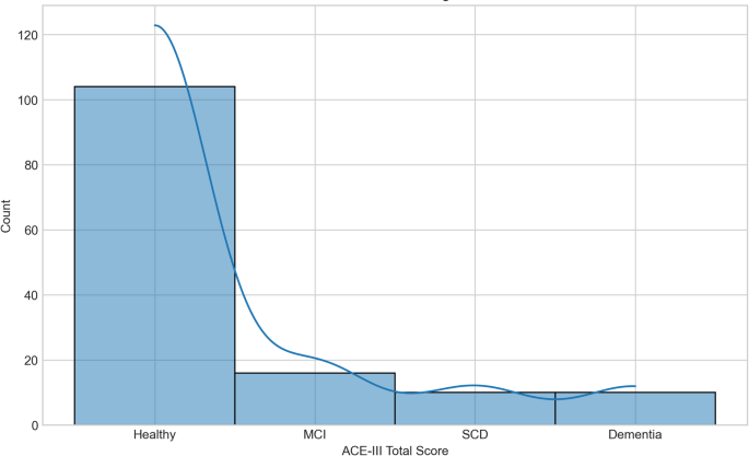
Target class distribution showing sample counts per cognitive category.
Data preprocessing pipeline
Continuous features were median-imputed and standardised (zero mean, unit variance). Categorical variables were mode-imputed and one-hot encoded with handle_unknown=’ignore’. These imputation, scaling, and encoding steps were fit on the full dataset prior to cross-validation; SMOTE (Sect. 3.5) was fit separately within each training fold only, so synthetic samples never touched validation data. As the dataset contains no missing values, the imputation steps have no practical effect regardless of fit scope; the components sensitive to the global fit are the standardisation of the single continuous feature (age) and the enumeration of one-hot categories, both expected to vary negligibly between a fold’s training partition and the full 140-participant sample. Nesting all preprocessing steps within-fold, as SMOTE already is, is recommended for future replications of this pipeline.
Fig. 3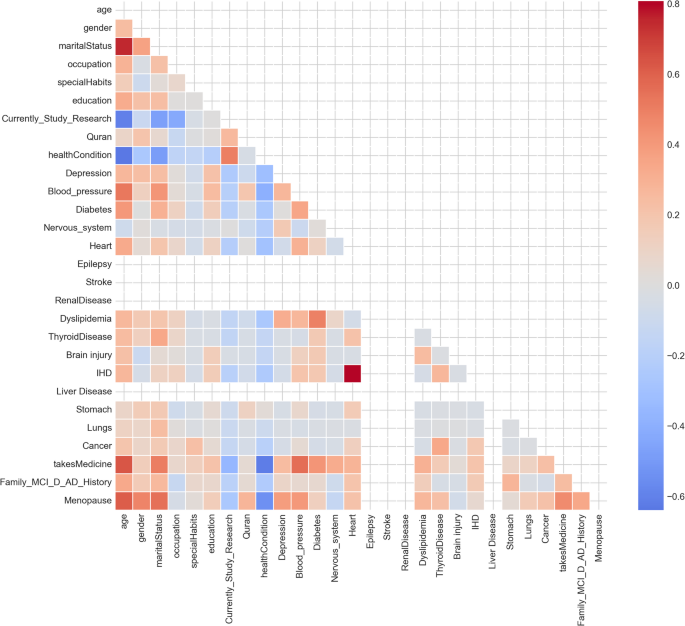
Pearson correlation heatmap of all 28 input features.
Feature distributions across cognitive groups
Figure 4 shows feature distributions broken down by cognitive group. Age climbs from CN through SCD and MCI to Dementia; education runs the opposite direction; depression and health burden increase with severity. These gradients align with what Egyptian clinicians observe in practice and confirm that the feature set is capturing real signal before any model has been fitted.
Class imbalance mitigation via SMOTE
SMOTE (k_neighbors = 2) was applied inside each training fold using an ImbPipeline, so synthetic samples from minority classes never touched the validation data. The value of k_neighbors was selected via a sensitivity sweep across the full feasible range (k = 1–7, bounded by the smallest per-fold minority class training count of 8): k = 2 achieved macro F1 in the top-performing tier (0.723, tied with k = 3) while showing more stable fold-to-fold performance on the SCD class specifically. We additionally compared SMOTE against ADASYN and Borderline-SMOTE across their own feasible neighbor-count ranges; no oversampler consistently outperformed the others, with all three producing macro F1 within a comparable band across configurations. Given that these estimates rest on only five folds and 10 real patients per minority class, we treat these small differences as fold-to-fold noise rather than a principled basis for preferring one configuration over another, consistent with the same reasoning applied to classifier hyperparameters in Sect. 3.6, and retain SMOTE with k_neighbors = 2 as a standard, conservative default. Figure 5 shows the before-and-after class frequencies: the 10:1 imbalance levels out. Applying SMOTE before the CV loop a common mistake in the published literature allows synthetic samples derived partly from validation instances to contaminate training, producing inflated estimates. We did not do that. SMOTE equalises minority class frequencies (MCI, SCD, Dementia) to match the Cognitively Normal majority, providing balanced training signal for all classifiers. SMOTE is applied exclusively within each training fold to prevent information leakage from validation data.
Fig. 4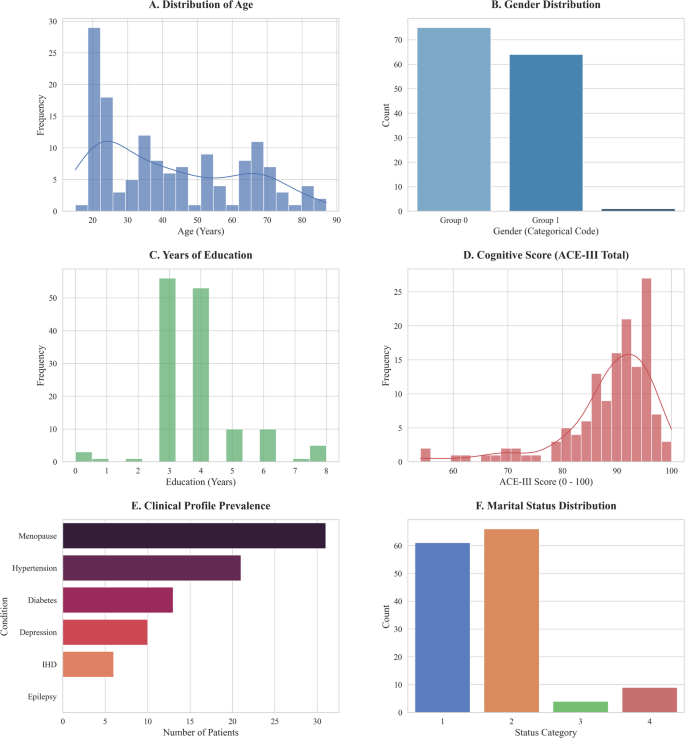
Exploratory data analysis: distribution of key clinical features across cognitive groups.
Machine Learning Algorithms
Twelve classifiers were evaluated on default hyperparameters unless noted: Logistic Regression (L2, class_weight=’balanced’); SVM with RBF kernel (probability calibration on); Decision Tree, Random Forest (100 trees), Extra Trees (100 trees), all balanced; XGBoost (mlogloss), LightGBM (leaf-wise), Gradient Boosting; Gaussian Naïve Bayes; KNN (k = 5); a soft-voting ensemble of RF + XGBoost + LightGBM + SVM; and a stacking classifier using RF + XGBoost + SVM as base learners with Logistic Regression as the meta-learner. Using defaults was deliberate: with a sample of this size, large-scale hyperparameter tuning risks fitting fold-specific noise rather than generalisable signal, and would disproportionately favour higher-capacity models (for example, LightGBM’s leaf-wise growth under an untuned num_leaves = 31 already has more effective capacity than, say, logistic regression) simply because they have more free parameters to exploit that noise. Evaluating all twelve classifiers on default settings therefore represents a conservative, fair benchmarking strategy: it avoids letting per-model tuning effort become a confound in the very model comparison this study is designed to make, at the acknowledged cost of not showing each algorithm’s ceiling performance.
Fig. 5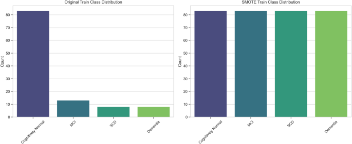
Training set class distribution before (left) and after (right) SMOTE resampling within a representative cross-validation fold.
Experimental framework and cross-validation protocol
Five-fold stratified cross-validation (random_state = 42) was used throughout. Figure 6 shows PCA and t-SNE projections of the original and SMOTE-resampled training data. SCD and MCI overlap heavily in both not surprising given how similar they are clinically, but it sets realistic expectations for classifier performance on those two classes. Substantial cluster overlap between SCD and MCI classes in both embeddings reflects the inherent phenotypic similarity of early cognitive decline stages, anticipating classification difficulty for these minority classes. Post-SMOTE embeddings demonstrate more balanced class representation without introducing artificial cluster separation.
UMAP embeddings
UMAP (Fig. 7) shows more structure than PCA: the CN and Dementia clusters are visibly more distinct, consistent with their more divergent clinical profiles and anticipating the higher per-class AUC values in the ROC analysis. UMAP preserves both local and global data structure, revealing more distinct class cluster formation than linear PCA particularly for the Cognitively Normal and Dementia classes. Greater inter-class separation in UMAP space for advanced cognitive stages is consistent with their more distinctive clinical profiles and anticipates their higher discriminative AUC values in classifier evaluation.
Evaluation metrics
Six metrics were computed on each held-out fold, macro-averaged across four classes: accuracy, macro F1-score (primary), one-vs-rest ROC-AUC, balanced accuracy, Cohen’s Kappa, and MCC. F1 was the primary metric: it balances precision and recall and is not inflated by the 74% majority class. Macro-averaging was chosen over a clinically weighted scheme because, unlike Cognitively Normal versus everything-else screening, no single misclassification direction among SCD, MCI, and Dementia is uniformly more costly in this four-class setting: under-calling a Dementia patient as MCI delays intervention, but over-calling an SCD patient as MCI or Dementia risks unnecessary patient anxiety and downstream testing, and clinical opinion on the relative severity of these errors varies by care setting and available resources. Macro F1-score treats all four classes, and by extension all types of misclassification, as equally important regardless of their prevalence, which we consider the more defensible default in the absence of a validated, setting-specific cost matrix; per-class F1, precision, and recall are reported separately (Sect. 4.6, Fig. 11) so that a deployment site with a specific cost structure in mind, for example one that weights missed Dementia cases more heavily, can weight these per-class results accordingly rather than relying on our aggregate choice.
Fig. 6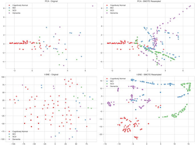
Two-dimensional embedding visualisations of original (top row) and SMOTE-resampled (bottom row) training data using Principal Component Analysis (PCA, left) and t-Distributed Stochastic Neighbour Embedding (t-SNE, right).
Fig. 7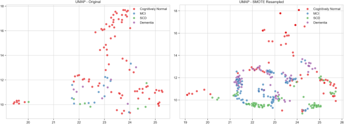
UMAP embeddings of original (left) and SMOTE-resampled (right) training data.
Let \(\:C=4\) denote the number of classes, \(\:N\) the total number of samples, and \(\:{\text{Conf}}_{kl}\)the number of samples with true class \(\:k\)predicted as class \(\:l\). For each class \(\:k\), \(\:T{P}_{k}\), \(\:F{P}_{k}\), and \(\:F{N}_{k}\) denote the true positives, false positives, and false negatives obtained from the one-vs-rest confusion matrix.
Accuracy is the proportion of correctly classified samples:
$$\:\text{Accuracy}=\frac{\sum\:_{k=1}^{C}{\text{Conf}}_{kk}}{N}$$
(1)
Macro F1-score is the unweighted mean of the per-class F1-scores, each computed from per-class precision and recall42:
$$\:{\text{Precision}}_{k}=\frac{T{P}_{k}}{T{P}_{k}+F{P}_{k}},\:{\text{Recall}}_{k}=\frac{T{P}_{k}}{T{P}_{k}+F{N}_{k}}$$
(2)
$$\:\begin{array}{cccc}&\:F{1}_{k}=\frac{2*{\text{Precision}}_{k}*{\text{Recall}}_{k}}{{\text{Precision}}_{k}+{\text{Recall}}_{k}}&\:&\:\end{array}$$
(3)
$$\:\text{Macro-F1}=\frac{1}{C}\sum\:_{k=1}^{C}F{1}_{k}$$
(4)
One-vs-rest ROC-AUC was computed by binarizing each class against the rest and averaging the resulting per-class areas under the ROC curve43:
$$\:\begin{array}{cccc}&\:\text{Macro\:ROC-AUC}=\frac{1}{C}\sum\:_{k=1}^{C}{\text{AUC}}_{k}&\:&\:\end{array}$$
(5)
Balanced accuracy is the mean of per-class recall (sensitivity), which corrects for class imbalance by weighting all classes equally regardless of their support44:
$$\:\begin{array}{cccc}&\:\text{Balanced\:Accuracy}=\frac{1}{C}\sum\:_{k=1}^{C}\frac{T{P}_{k}}{T{P}_{k}+F{N}_{k}}&\:&\:\end{array}$$
(6)
Cohen’s Kappa measures agreement between predicted and true labels beyond what would be expected by chance45:
$$\:\begin{array}{cccc}&\:\kappa\:=\frac{{p}_{o}-{p}_{e}}{1-{p}_{e}}&\:&\:\end{array}$$
(7)
where \(\:{p}_{o}\) is the observed accuracy and \(\:{p}_{e}\) is the expected agreement by chance, computed from the marginal totals of the confusion matrix:
$$\:\begin{array}{cccc}&\:{p}_{o}=\frac{\sum\:_{k=1}^{C}{\text{Conf}}_{kk}}{N},\:{p}_{e}=\sum\:_{k=1}^{C}\left(\frac{{\text{row}}_{k}}{N}\right)\left(\frac{{\text{col}}_{k}}{N}\right)&\:&\:\end{array}$$
(8)
with \(\:{\text{row}}_{k}={\sum\:}_{l}{\text{Conf}}_{kl}\) and \(\:{\text{col}}_{k}={\sum\:}_{l}{\text{Conf}}_{lk}\) denoting the true and predicted totals for class \(\:k\), respectively.
Matthews Correlation Coefficient (MCC) was computed using its multiclass generalization46:
$$\:\begin{array}{cccc}&\:MCC=\frac{c\cdot\:s-\sum\:_{k=1}^{C}{p}_{k}{t}_{k}}{\sqrt{\left({s}^{2}-\sum\:_{k=1}^{C}{p}_{k}^{2}\right)\left({s}^{2}-\sum\:_{k=1}^{C}{t}_{k}^{2}\right)}}&\:&\:\end{array}$$
(9)
where \(\:c={\sum\:}_{k=1}^{C}{\text{Conf}}_{kk}\) is the total number of correct predictions, \(\:s=N\) is the total number of samples, \(\:{p}_{k}={\sum\:}_{l}{\text{Conf}}_{lk}\) is the number of times class \(\:k\) was predicted, and \(\:{t}_{k}={\sum\:}_{l}{\text{Conf}}_{kl}\) is the number of times class \(\:k\) actually occurred. MCC ranges from \(\:-1\) to \(\:1\), with \(\:0\) indicating random prediction, and is considered robust to class imbalance since it accounts for all four cells of the confusion matrix simultaneously.
\(\:c={\sum\:}_{k=1}^{C}{\text{Conf}}_{kk}\)(total correct predictions).
\(\:s=N\)(total samples).
\(\:{p}_{k}={\sum\:}_{l=1}^{C}{\text{Conf}}_{lk}\)(times class \(\:k\)was predicted).
\(\:{t}_{k}={\sum\:}_{l=1}^{C}{\text{Conf}}_{kl}\)(times class \(\:k\)actually occurred).
Statistical inference
LightGBM was compared against each competitor using paired t-tests on the five fold-level F1-scores (threshold: \(\:p<0.05\)). Wilcoxon signed-rank tests provided non-parametric cross-checks. McNemar’s test was planned for per-sample error analysis.
For each competing model, let \(\:{d}_{i}=F{1}_{i}^{\text{L}\text{i}\text{g}\text{h}\text{t}\text{G}\text{B}\text{M}}-F{1}_{i}^{\text{comp}}\) denote the difference in fold-level macro-F1 scores for fold \(\:i\), \(\:i=1,\dots\:,5\). The paired t-test statistic is47:
$$\:\begin{array}{cccc}&\:t=\frac{\stackrel{-}{d}}{{s}_{d}/\sqrt{n}}&\:&\:\end{array}$$
(10)
where \(\:\stackrel{-}{d}\) is the mean of the paired differences, \(\:{s}_{d}\) is their standard deviation, and \(\:n=5\) is the number of folds. Under the null hypothesis of no difference in performance, \(\:t\)follows a \(\:t\)-distribution with \(\:n-1\) degrees of freedom.
The Wilcoxon signed-rank test ranks the absolute differences \(\:\mid\:{d}_{i}\mid\:\) and sums the ranks associated with positive differences48:
$$\:\begin{array}{cccc}&\:W=\sum\:_{i=1}^{n}\text{sgn}\left({d}_{i}\right)\cdot\:{R}_{i}&\:&\:\end{array}$$
(11)
where \(\:{R}_{i}\) is the rank of \(\:\mid\:{d}_{i}\mid\:\) among all \(\:\mid\:{d}_{1}\mid\:,\dots\:,\mid\:{d}_{n}\mid\:\), and \(\:\text{sgn}\left({d}_{i}\right)\) is \(\:+1\) if \(\:{d}_{i}>0\) and \(\:-1\) if \(\:{d}_{i}<0\).
McNemar’s test compares per-sample errors between two classifiers using a 2 × 2 contingency table of discordant predictions, where \(\:b\) is the number of samples LightGBM classified correctly but the competitor misclassified, and \(\:c\)is the reverse49:
$$\:\begin{array}{cccc}&\:{\chi\:}^{2}=\frac{{\left(b-c\right)}^{2}}{b+c}&\:&\:\end{array}$$
(12)
which follows a \(\:{\chi\:}^{2}\) distribution with 1 degree of freedom under the null hypothesis that both classifiers have the same error rate.
SHAP explainability framework
SHAP estimators were matched to model type: TreeExplainer (exact) for all tree-based models, KernelExplainer for SVM and KNN, LinearExplainer for Logistic Regression. All three approximate the same underlying quantity, the Shapley value, but differ in how they estimate it efficiently for a given model class50.
For a model \(\:f\) trained on a feature set with \(\:M\)total features, the Shapley value \(\:{\phi\:}_{i}\) for feature \(\:i\)on a given prediction is defined as:
$$\:\begin{array}{cccc}&\:{\phi\:}_{i}=\sum\:_{S\subseteq\:M\setminus\:\left\{i\right\}}\frac{\mid\:S\mid\:!\text{\hspace{0.17em}}\left(M-\mid\:S\mid\:-1\right)!}{M!}[{f}_{x}\left(S\cup\:\left\{i\right\}\right)-{f}_{x}\left(S\right)]&\:&\:\end{array}$$
(13)
where \(\:S\)ranges over all subsets of features excluding \(\:i\), and \(\:{f}_{x}\left(S\right)\) is the model’s expected output when only the features in \(\:S\)are known. Each \(\:{\phi\:}_{i}\) represents feature \(\:i\)‘s marginal contribution to the prediction, averaged over every possible ordering in which features could be added50.
Mean absolute SHAP values were used to rank global feature importance across the validation set. For feature \(\:i\) across \(\:n\) validation samples:
$$ \left| {\overline{\phi } _{i} } \right| = \frac{1}{n}\sum\limits_{{j = 1}}^{n} {\left| {\phi _{i}^{{\left( j \right)}} } \right|} $$
(14)
where \(\:{\phi\:}_{i}^{\left(j\right)}\) is the Shapley value of feature \(\:i\) for sample \(\:j\). Features were ranked in descending order of \( \left| {\overline{\phi } _{i} } \right| \) for each of the three estimator types.
The key finding is that top-ranked features are consistent across all three estimator types, which is the strongest available evidence that they reflect real clinical signal rather than estimation artefacts.
Reproducibility
All random seeds fixed at 42. Software: Python 3.9.6, scikit-learn 1.6.1, XGBoost 2.1.4, LightGBM 4.6.0, imbalanced-learn 0.12.4, SHAP 0.49.1. Runtime: roughly 25–40 min on standard CPU. The pipeline can be run directly on any comparable Egyptian Arabic ACE-III dataset. Experiments were run on macOS-26.5.1-x86_64-i386-64bit. RAM was not logged, as psutil was not installed in the runtime environment. No GPU was used; all computation ran on CPU with n_jobs = 1.