
Electric control of energy detuning
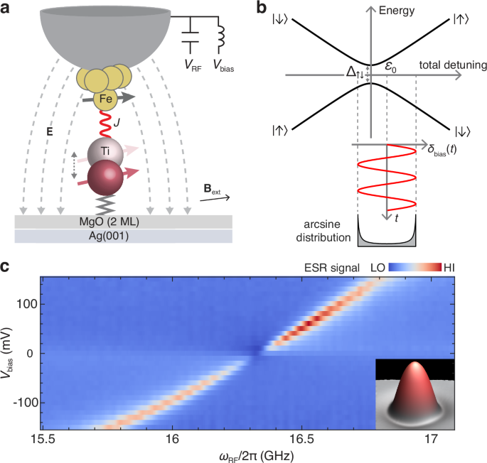
The Ti atoms were deposited on the two-monolayer MgO film grown on Ag(001), and are electrically accessible by measuring the time-averaged tunnel current24. The MgO serves as a decoupling layer, which increases the coherence time of the Ti spins24,25. We focus on spin-1/2 Ti atoms adsorbed at the bridge site between two oxygen atoms of MgO26. The spin-polarized STM tip, prepared by transferring Fe atoms to the tip apex, is used to probe and control the Ti spins. Single-atom ESR signals are measured by applying a bias voltage \({V}_{{{\rm{bias}}}}\) and an RF voltage \({V}_{{{\rm{RF}}}}\) of frequency \({\omega }_{{{\rm{RF}}}}\) across the STM tunnel junction21,24.
The magnetic field experienced by a Ti spin (S) is the vector sum of the externally applied field \({{{\bf{B}}}}_{{{\rm{ext}}}}\) and the effective field of the tip27. The tip field is modulated by \({V}_{{{\rm{RF}}}}\), and thus has a static component \({{{\bf{B}}}}_{{{\rm{tip}}}}\) and an oscillatory component\(\,\Delta {{{\bf{B}}}}_{{{\rm{tip}}}}\cos ({\omega }_{{{\rm{RF}}}}t)\). The Hamiltonian is therefore given by21,27:
$$H=g{\mu }_{{{\rm{B}}}}{{\bf{B}}}\cdot {{\bf{S}}}+g{\mu }_{{{\rm{B}}}}\Delta {{{\bf{B}}}}_{{{\rm{tip}}}}\cdot {{\bf{S}}}\cos \left({\omega }_{{{\rm{RF}}}}t\right)\,\,$$
(1)
where \({{\bf{B}}}={{{\bf{B}}}}_{{{\rm{ext}}}}+{{{\bf{B}}}}_{{{\rm{tip}}}}\) is the total static field, which sets the Zeeman splitting between the spin-up \(\left|\uparrow \right\rangle\) and spin-down \(\left|\downarrow \right\rangle\) states. The g-factor is about 1.8, and \({\mu }_{B}\) is the Bohr magneton24,26.
Realizing LZSM interference requires two key ingredients28. One is the avoided level crossing, which can be obtained by making a transformation into a frame rotating with frequency \({\omega }_{{{\rm{RF}}}}\). In the rotating frame, the oscillatory tip field becomes a static transverse magnetic field, which hybridizes the \(\left|\uparrow \right\rangle\) and \(\left|\downarrow \right\rangle\) states, opening an anticrossing of magnitude \({\Delta }_{\uparrow \downarrow }={{\hslash }}{\Omega }_{{{\rm{Rabi}}}}\) at zero energy detuning (Fig. 1b), where \({\Omega }_{{{\rm{Rabi}}}}\) is the Rabi frequency.
The second ingredient is an adjustable energy detuning, which sets the energy difference between the \(\left|\uparrow \right\rangle\) and \(\left|\downarrow \right\rangle\) states. We controlled the detuning of the spin-1/2 Ti atom by the bias voltage \({V}_{{{\rm{bias}}}}\), which induces a very strong electric field as high as ~1 GV/m across the STM junction due to the sub-nanometer tip-sample distance19,27,29. In turn, this results in a modulation of the spin splitting of the surface spin, which we probe using ESR-STM. Specifically, we measure the evolution of ESR spectra of a single Ti spin as a function of \({V}_{{{\rm{bias}}}}\), taken at a constant static tip-atom distance (Fig. 1c)19. The ESR peak shifts almost linearly with \({V}_{{{\rm{bias}}}}\). As the ESR frequency is proportional to \({B}_{{{\rm{ext}}}}+{B}_{{{\rm{tip}}}}\), this frequency shift indicates that \({B}_{{{\rm{tip}}}}\) increases monotonically with increasing \({V}_{{{\rm{bias}}}}\), giving rise to an effective detuning shift of ~2-4 MHz/mV depending on the STM tip.
The spin-electric field coupling may arise from an atomic-scale piezoelectric effect, where the strong electric field alters the equilibrium position of the Ti atom on MgO by ~1% of the Ti-MgO distance19,27,29. Since the spin interaction between the magnetic tip and the Ti atom depends exponentially on their distance27, the piezoelectric displacement of the Ti atom results in a modified static \({B}_{{{\rm{tip}}}}\) and thus the energy detuning (Fig. 1a). Since the displacement (~1 pm) is much smaller than the decay length (~ 0.4 Å) of the spin interaction19,27, the energy detuning depends approximately linearly on the bias voltage (Fig. 1c). This electrical spin control of energy detuning offers architectural advantages for quantum spintronics because electric fields can be efficiently routed and confined in nanoscale circuits and adjusted faster compared to magnetic fields2,19,30.
We can thus obtain a modulation \({\delta }_{{{\rm{bias}}}}(t)\) of the energy detuning by adding a time-varying component to \({V}_{{{\rm{bias}}}}\) (Fig. 1a). In the rotating frame, the spin Hamiltonian under \({V}_{{{\rm{RF}}}}\) and modulated \({V}_{{{\rm{bias}}}}\) is written as:
$$H=\left[{\varepsilon }_{0}+{\delta }_{{{\rm{bias}}}}(t)\right]{S}_{z}+{\Delta }_{\uparrow \downarrow }{S}_{x}$$
(2)
where the static detuning \({\varepsilon }_{0}={{\hslash }}\left({\omega }_{0}-{\omega }_{{{\rm{RF}}}}\right)\), and \({\omega }_{0}=g{\mu }_{{{\rm{B}}}}B/{{\hslash }}\) denotes the Larmor frequency. Here z-axis is the spin quantization axis as determined by the direction of the total static field \({{\bf{B}}}\).
LZSM interference of single spins
Our pulse sequence for LZSM measurement is illustrated in Fig. 2a. A bias voltage is applied at the tip-atom junction, with a sinusoidal modulation \({V}_{{{\rm{bias}}}}(t)={V}_{{{\rm{DC}}}}+\delta V\sin \left(2{{\rm{\pi }}}{ft}\right)\), on top of the RF voltage, with frequency \(f\ll {\omega }_{{{\rm{RF}}}}/2{{\rm{\pi }}}\). Here \({V}_{{{\rm{DC}}}}\) is the DC bias voltage; \(\delta V\) and \(f\) are the modulation amplitude and frequency, respectively. The modulated bias voltage \({V}_{{{\rm{bias}}}}(t)\) drives the Ti spin repeatedly through the avoided level crossing (Fig. 1b), and we probe its effect on the steady-state spin occupation using single-atom ESR, which is sensitive to the change of spin population21,24. Figure 2b shows the LZSM pattern as a function of modulation frequency \(f\) and static detuning \({\varepsilon }_{0}\) \(\propto \left({\omega }_{{{\rm{RF}}}}-{\omega }_{0}\right)\). For each static detuning, we measured the ESR signal at different modulation frequencies (Fig. 1b). The tunnel current shows clear LZSM interference fringes as a result of the phase accumulation between consecutive Landau-Zener transitions1.
Fig. 2: LZSM interference of a single Ti spin.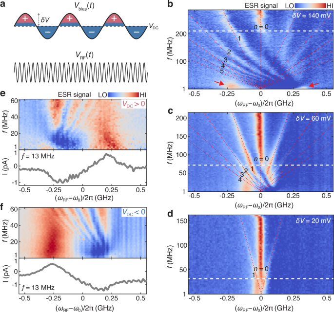
a Schematics of the pulse sequences for the LZSM measurement. Both \({V}_{{{\rm{bias}}}}\) and \({V}_{{{\rm{RF}}}}\) are sinusoidal in time. \({V}_{{{\rm{DC}}}}\) and \(\delta V\) are the DC component and modulation amplitude of \({V}_{{{\rm{bias}}}}\). The polarity of \({V}_{{{\rm{bias}}}}\) is indicated by + (red regions) and – (blue regions) signs. b–d ESR spectra as a function of detuning \({\omega }_{{{\rm{RF}}}}-{\omega }_{0}\) and modulation frequency \(f\), measured at a fixed modulation amplitude \(\delta V\) of 140, 60 and 20 mV, respectively (\({V}_{{{\rm{DC}}}}\) = −50 mV, \({V}_{{{\rm{RF}}}}\) = 20 mV; \({B}_{{{\rm{ext}}}}\) = 0.58 T; setpoint: \({V}_{{{\rm{sp}}}}\) = 50 mV, \({I}_{{{\rm{sp}}}}\) = 60 pA). The multiphoton resonances at \(\left|{\omega }_{{{\rm{RF}}}}-{\omega }_{0}\right|/2{{\rm{\pi }}}={nf}\) are labeled, and also indicated by red dashed lines. Dashed white lines indicate the onset of motional averaging. Red arrows in b indicate the two main peaks at slow modulation. The detuning shift is ~1.9 MHz/mV for the STM tip used. e, f ESR spectra measured at low modulation frequencies \(f\) with positive (e) and negative (f) DC voltages \({V}_{{{\rm{DC}}}}\) (\({V}_{{{\rm{DC}}}}\) = 50, −40 mV, \(\delta V\) = 100, 80 mV, \({V}_{{{\rm{RF}}}}\) = 15 mV; \({B}_{{{\rm{ext}}}}\) = 0.52 T; setpoint: \({V}_{{{\rm{sp}}}}\) = 50 mV, \({I}_{{{\rm{sp}}}}\) = 50 pA). The lower panels show the ESR spectra at \(f\) = 13 MHz.
The LZSM patterns in Fig. 2b exhibit various spectroscopic features depending on how fast the spin is driven, which according to our model (Supplementary Note 2), are governed by the dimensionless parameter \(2{{\rm{\pi }}}f{T}_{2}\). In the slow limit \((2{{\rm{\pi }}}f{T}_{2}\ll 1)\), that corresponds to \(f\) < 10 MHz, the spectra exhibit two main ESR peaks (red arrows in Fig. 2b). This regime can be interpreted as if we were performing conventional ESR-STM experiments, but with a range of resonance frequencies following an arcsine distribution (Fig. 1b). In contrast, the interference pattern is observed in the coherent limit (\(f\) > 20 MHz), where consecutive traversals of anticrossing take place within the spin coherence time T2. In this regime, a complex pattern with additional sidebands is observed. These ESR side peaks, appearing at \(\left|{\omega }_{{{\rm{RF}}}}-{\omega }_{0}\right|/2{{\rm{\pi }}}={nf}\), correspond to excitation processes driven by the adsorption of \(n\) photons (\(n\le 5\), see Fig. 2b)1. The dressed spin is resonantly excited when the dressed energy splitting \({{\hslash }}\left|{\omega }_{{{\rm{RF}}}}-{\omega }_{0}\right|\) matches the energy of n-photon (Supplementary Note 1). The observation of the multiphoton process requires a very high driving field, which is easily fulfilled in the STM junction due to the sub-nanometer tip-atom distance. Note that the spectrum should exbibit a single resonant peak at zero modulation frequency, but once the modulation frequency becomes non-zero, the resonance frequency follows an arcsine distribution in the slow modulation limit.
Further increasing the modulation frequency \(f\), a strong ESR peak appears at zero static detuning (\({\omega }_{{{\rm{RF}}}}{=\omega }_{0}\)), which corresponds to the motional average of the two main peaks at small modulation frequency31,32.
We further studied the dependence of the LZSM spectra on the modulation amplitude \(\delta V\) (Fig. 2b–d). The two main peaks at small modulation frequencies (\(f\)) roughly correspond to the two different resonance values, \({B}_{{{\rm{ext}}}}+{B}_{{{\rm{tip}}}}(+\delta V)\) and \({B}_{{{\rm{ext}}}}+{B}_{{{\rm{tip}}}}(-\delta V)\). As expected from the quasi-linear relation between \({B}_{{{\rm{tip}}}}\) and \(\delta V\), as \(\delta V\) increases, the energy difference of the two main peaks reached by the energy detuning modulation also increases (Fig. 2b–d). Consequently, the frequency \(f\) above which the motional average is effective increases with larger \(\delta V\), as indicated by the dashed white lines in Fig. 2b–d. This can be rationalized in terms of the energy-time uncertainty32. In addition, as the modulation amplitude \(\delta V\) increases, higher-order ESR side peaks become more visible, indicating higher-order photon modes increasingly participate in the excitation process, while the energy separation between adjacent photon-assisted modes is independent of \(\delta V\).
We also measured the LZSM interference as a function of driving amplitudes \(\delta V\) for a fixed modulation frequency \(f\), and observed multiphoton resonances within a V-shaped region (Supplementary Fig. 1), as the driving amplitude needs to be large enough to reach the avoided level crossing (Fig. 1b).
Spin-transfer torque in LZSM interference
As shown in Fig. 2b, the LZSM spectra exhibit pronounced asymmetries with respect to zero static detuning (\({\omega }_{{{\rm{RF}}}}={\omega }_{0}\)), which cannot be captured by the conventional LZSM theory1, and is in contrast to the symmetric patterns observed in other quantum systems2,3,4,7.
This asymmetric pattern results from the spin-transfer torque on the Ti atom under the influence of the spin-polarized tunnel current20,22,33. The spin-transfer torque process is illustrated in Fig. 3a. At a positive \({V}_{{{\rm{bias}}}}\), the inelastic tunneling electron (\(\Delta \sigma=+ 1\)) is able to cause a spin flip of the Ti atom (\(\Delta {m}_{{{\rm{Ti}}}}=-1\)) as the total spin angular momentum is conserved during the spin-scattering event. Reversing the polarity of \({V}_{{{\rm{bias}}}}\) and thus the direction of tunnel current drives the Ti spin to the opposite direction (\(\Delta {m}_{{{\rm{Ti}}}}=+ 1\)).
Fig. 3: Simulation of the LZSM interference by considering the spin-transfer torque effects using the generalized Bloch equations.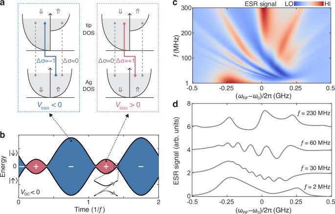
a Schematic of the spin-transfer torque on the Ti atom under the influence of spin-polarized tunnel current at different bias polarities, showing \(\Delta {{\rm{\sigma }}}=+ 1\) (red arrow), \(\Delta {{\rm{\sigma }}}=-1\) (blue arrow), and \(\Delta {{\rm{\sigma }}}=0\) (dashed arrows) electron tunneling between the spin-dependent (⇑ or ⇓) densities of states (DOS) of Ag and STM tip. The bias is given with respect to the sample. b Time evolution of energy levels of the Ti spin driven by bias voltage modulation for \({V}_{{\mbox{DC}}}\) < 0. The polarity of \({V}_{{{\rm{bias}}}}\) is indicated by + (red regions) and – (blue regions) signs. c Simulated ESR signals as a function of detuning \({\omega }_{{{\rm{RF}}}}-{\omega }_{0}\) and modulation frequency \(f\) for a fixed modulation amplitude \(\delta V\) of 140 mV. Simulations parameters: \({\omega }_{0}\) = 15.5 GHz, ∆↑↓ = 40 MHz, \({\delta }_{{{\rm{bias}}}}\left(t\right)=273\sin (2{{\rm{\pi }}}ft)\) MHz, \({V}_{{\mbox{DC}}}=-50\) mV, \(\eta\) = \(3.5\times {10}^{-5}\), \(\alpha\) = 0.5, \({\left\langle {S}_{z}\right\rangle }_{0}\) = −0.18, \(\left\langle {S}_{{{\rm{tip}}}}^{z}\right\rangle\) = 1, \(\left\langle {S}_{{{\rm{tip}}}}^{{xy}}\right\rangle\) = 0.5, \({\left\langle {S}_{{{\rm{z}}}}^{{{\rm{p}}}}\right\rangle }_{0 ,{{\rm{STT}}}}=-0.2\), \({\left\langle {S}_{{{\rm{z}}}}^{{{\rm{n}}}}\right\rangle }_{0 ,{{\rm{STT}}}}=0.3\), \(k=0.01\), \({V}_{{\mbox{RF}}}\) = 20 mV, \({T}_{1}^{{\mathrm{int}}}=161\,{{\rm{ns}}} ,\,{T}_{2}^{{\mathrm{int}}}=\,322\,{{\rm{ns}}}\). See Supplementary Note 2 for the meaning of each parameter. d Simulated ESR signals at \(f=\) 2, 30, 60 and 230 MHz, respectively.
During the quantum interference, the atomic-scale spin-transfer torque process competes with the energy-level modulation (Fig. 3b). Since the center bias voltage \({V}_{{{\rm{DC}}}}\) of \({V}_{{{\rm{bias}}}}\) is nonzero, the amplitude of the spin-polarized current at positive \({V}_{{{\rm{bias}}}}\) (indicated by + in Figs. 2a and 3b) differs from that at the negative \({V}_{{{\rm{bias}}}}\) (indicated by − in Figs. 2a and 3b). This makes the symmetry of the LZSM pattern highly dependent on the polarity of \({V}_{{{\rm{DC}}}}\), and the LZSM pattern is flipped with respect to \({\omega }_{{{\rm{RF}}}}{=\omega }_{0}\) as the polarity of \({V}_{{{\rm{DC}}}}\) is reversed (Supplementary Fig. 2).
To quantitatively understand the asymmetric LZSM pattern, we calculate the time evolution of the periodically driven Ti spin using the generalized Bloch equations, and consider coherent driving, spin relaxation and decoherence, as well as the effect of spin-transfer torque by tunneling electrons during the energy-level modulation (Supplementary Note 2). The simulation results (Fig. 3c and Supplementary Fig. 3) agree well with the measured asymmetric LZSM pattern. As shown in Fig. 3c, d, the simulation reproduces the evolution from the two main peaks under very slow modulation, to the peak-dip spectra as well as asymmetric stripe patterns, and eventually to the more symmetric interference patterns at the high-\(f\) regime. The agreement between the experiment and the simulation suggests that the observed side bands and interference fringes are not due to higher harmonics of the modulation.
The spectroscopic asymmetry is more pronounced in the low-\(f\) regime (\(f \sim 5-20{{\rm{MHz}}}\)) of the LZSM spectra, where it manifests as a peak-dip lineshape in the ESR spectra (Figs. 2e, f and 3c, d). The dip occurs because the change in spin-state population, driven by the spin-transfer torque, cannot keep up with the rapid bias voltage modulation. This could occur for certain bias polarity during the modulation cycle, for example, the positive bias cycle in Fig. 2f where the center bias voltage \({V}_{{{\rm{DC}}}}\) is negative, leading to the dip in the spectra at \({\omega }_{{{\rm{RF}}}} > {\omega }_{0}\). In contrast, for the negative bias cycle, spin-state population could still reach the nonequilibrium set by the larger negative spin-polarized current, resulting in the ESR peak.
When the bias voltage modulation is much faster than the spin relaxation, the change of spin-state population induced by spin-transfer torque becomes almost negligible over each cycle of the rapid energy-level modulation, leading to a less asymmetric interference pattern (Figs. 2b–d and 3c, d).
The asymmetric LZSM patterns highlight the dissipative action of the spin transfer-torque during quantum infereference20. The presence of the spin-polarized current also leads to a nonequilibrium initialization of the Ti spin, and thus could overcome the thermal population constrains.
LZSM interferometry using frequency modulation
In addition to modulating the bias voltage as shown above, we are also able to perform LZSM interferometry using frequency-modulated RF voltage34. The frequency modulation of \({V}_{{{\rm{RF}}}}\) effectively modulates the fictitious field along the z-axis in the rotating frame, resulting in a tunable energy detuning. Compared to the bias voltage modulation, modulating the frequency of \({V}_{{{\rm{RF}}}}\) offers the advantage of achieving much larger energy detuning, and also reduces spin scattering of Ti atom by tunnel current, leading to a longer T2 time.
Specifically, we apply an RF voltage with modulated frequency \({\omega }_{{{\rm{RF}}}}\left(t\right)={\omega }_{{{\rm{RF}}}}+{\delta }_{{{\rm{RF}}}}\left(t\right)\) to the tunnel junction, where \({\omega }_{{{\rm{RF}}}}\) is the center frequency and \({\delta }_{{{\rm{RF}}}}\left(t\right)\) describes the frequency modulation. The corresponding spin Hamiltonian in the rotating frame is (Supplementary Note 3)
$$H=\left[{\varepsilon }_{0}-{\hslash \delta }_{{{\rm{RF}}}}\left(t\right)\right]{S}_{z}+{\Delta }_{\uparrow \downarrow }{S}_{x}$$
(3)
Figure 4b shows the LZSM interference pattern measured with a sinusoidal frequency modulation: \({\delta }_{{{\rm{RF}}}}\left(t\right)={\delta }_{{{\rm{RF}}}}\sin \left(2{{\rm{\pi }}}{ft}\right)\), where \({\delta }_{{{\rm{RF}}}}\) is the modulation amplitude (Fig. 4a). The frequency modulation results in a sinusoidal modulation of the energy detuning (Eq. (3)). The reduced linewidth of the ESR peaks compared to Fig. 2b–d is in line with both previous theory work1 and our numerical calculation, which show that for large values of \(2{{\rm{\pi }}}f{T}_{2}\), the linewidth is primarily governed by the Rabi coupling. This narrowing of the linewidth also suggests an improved T2 time due to a smaller averaged tunnel current flowing through the Ti atom. Importantly, a much larger energy detuning (~1 GHz) can be achieved compared to the bias voltage modulation, by simply increasing the frequency modulation amplitude \({\delta }_{{{\rm{RF}}}}\). This combination of reduced linewidth and larger energy detuning enables the observation of higher-order multiphoton resonances with up to 8 photons. Furthermore, the LZSM spectra become symmetric since a constant bias voltage is applied, thereby eliminating the influence of spin-transfer torque modulation. This symmetric pattern is well reproduced by our simulation (Fig. 4c). We also measured LZSM interference as a function of \({\delta }_{{{\rm{RF}}}}\) while keeping the modulation frequency \(f\) fixed, and observed symmetric patterns in V-shaped regions (Supplementary Fig. 4).
Fig. 4: LZSM interference measured with frequency modulation of VRF.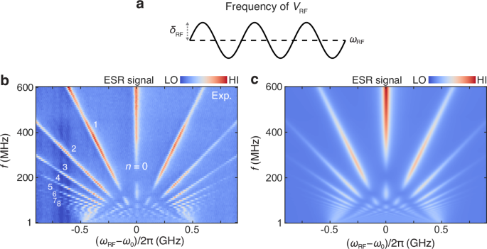
a Schematics of the pulse sequences for the LZSM measurement in (b). A sinusoidally frequency-modulated \({V}_{{{\rm{RF}}}}\) is used, with a center frequency \({\omega }_{{{\rm{RF}}}}\) and modulation amplitude \({\delta }_{{{\rm{RF}}}}\). b ESR spectra as a function of detuning \({\omega }_{{{\rm{RF}}}}-{\omega }_{0}\) and modulation frequency \(f\), measured using a sinusoidal frequency modulation of \({V}_{{{\rm{RF}}}}\) (\({\delta }_{{{\rm{RF}}}}\) = 0.5 GHz, \({V}_{{{\rm{RF}}}}\) = 10 mV, \({V}_{{{\rm{bias}}}}\) = 50 mV; \({B}_{{{\rm{ext}}}}\) = 0.60 T; setpoint: \({V}_{{{\rm{sp}}}}\) = 50 mV, \({I}_{{{\rm{sp}}}}\) = 30 pA). c Simulations of LZSM interference with frequency modulation of \({V}_{{{\rm{RF}}}}\) using the generalized Bloch equations. Simulations parameters: \({\omega }_{0}\) = 15.5 GHz, \({V}_{{\mbox{DC}}}=50\) mV, \({\delta }_{{{\rm{RF}}}}\) = 500\(\sin (2{{\rm{\pi }}}ft)\) MHz, \({\Delta }_{\uparrow \downarrow }\) = 20 MHz, \(\alpha\) = 0.5, \({\left\langle {S}_{z}\right\rangle }_{0}\) = −0.18, \(\left\langle {S}_{{{\rm{tip}}}}^{z}\right\rangle\) = 1, \(\left\langle {S}_{{{\rm{tip}}}}^{{xy}}\right\rangle\) = 0.5, \({V}_{{\mbox{RF}}}\) = 10 mV, \({T}_{1}=40\,{{\rm{ns}}} ,\,{T}_{2}=\,40\,{{\rm{ns}}}\).
In addition, using frequency modulation of VRF, we can realize quantum interference under more complex situations. For instance, we realized the quantum interference in a two-level system under the modulation of both energy detuning and avoided anticrossing, using two frequency-modulated RF components (Supplementary Fig. 8). This measurement provides new opportunities for quantum control, which is complementary to spin rotations using Rabi oscillations11,21.
The T2 time is mainly limited by tunneling current–induced decoherence21, and depends on excitation conditions. In the bias modulation scheme, increasing \(\delta V\) raises the averaged current when \(\delta V\) exceeds \({V}_{{{\rm{DC}}}}\), and thus reduces T2. In the RF frequency modulation scheme, the T2 time remains unaffected as the average current stays constant with increasing \({\delta }_{{{\rm{RF}}}}\). Substrate electron scattering also contributes to decoherence21, causing slight T2 variations among adatoms due to local environments.
LZSM interference of coupled spins
We further demonstrate LZSM interference in multi-level systems using two coupled Ti spins with tunable interaction. The LZSM patterns reveal spectroscopic information about the energy level diagrams of spin dimers, including the occurrence of avoided level crossings as well as the magnetic interaction, and can be utilized to characterize the many-body energy levels of more complex quantum magnets9,16,35.
The Ti spins are coupled by antiferromagnetic interaction (J > 0) (Fig. 5a), and the eigenstates consist of spin singlet state \(\left|{{\rm{S}}}\right\rangle\) and triplet states \(\left|{{{\rm{T}}}}_{+}\right\rangle\), \(\left|{{{\rm{T}}}}_{0}\right\rangle\) and \(\left|{{{\rm{T}}}}_{-}\right\rangle\) (refs. 18,19,24,26). Similar to the single spin, \({V}_{{{\rm{bias}}}}\) can be used to control the energy detuning and thus the Zeeman energy of the spin \({{{\bf{S}}}}_{1}\) under the STM tip. As \({V}_{{{\rm{bias}}}}\) varies, the energy-level diagram exhibits an avoided level crossing between \(\left|{{\rm{S}}}\right\rangle\) and \(\left|{{{\rm{T}}}}_{0}\right\rangle\) (Fig. 5b), which is detected by ESR spectra measured on \({{{\bf{S}}}}_{1}\) (Fig. 5c). Unlike the single spin (Fig. 1c), the ESR frequencies of coupled spins (Ⅰ-IV) vary nonlinearly with \({V}_{{{\rm{bias}}}}\) due to the spin coupling. In the following, we tune the two spins to the maximal level of entanglement by adjusting \({V}_{{{\rm{bias}}}}\) to position the system at the anticrossing point (red dashed lines in Fig. 5b, c)18,24. At this point, the two spins experience the same Zeeman splitting and thus have the same Larmor frequency \({\omega }_{0}\).
Fig. 5: Tuning the LZSM interference of coupled spins.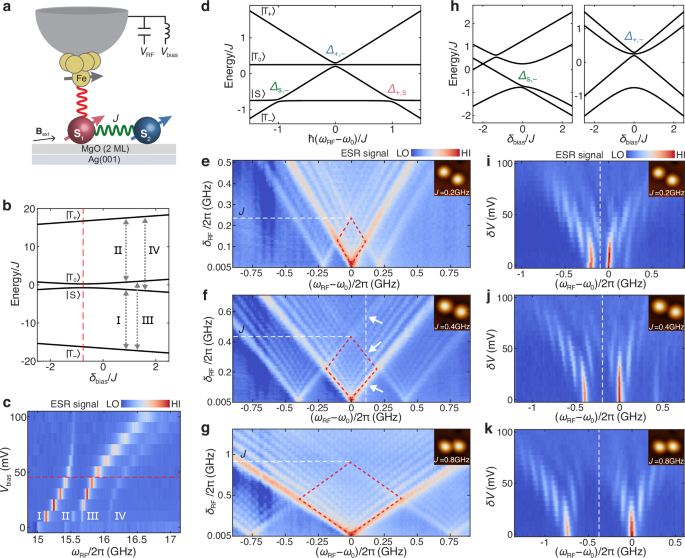
a Schematic showing two Ti spins with a coupling J (green curve). The tip-Ti coupling is indicated by the red curve. b Energy-level diagram of two spins as a function of the energy detuning \({\delta }_{{{\rm{bias}}}}\) due to \({V}_{{{\rm{bias}}}}\). \(\left|{{\rm{S}}}\right\rangle\) and \(\left|{{{\rm{T}}}}_{0}\right\rangle\) exhibit an anticrossing (red dashed line). c ESR spectra of a Ti spin dimer (J = 0.4 GHz) as a function of \({\omega }_{{{\rm{RF}}}}\) and \({V}_{{{\rm{bias}}}}\) (setpoint: \({V}_{{{\rm{sp}}}}\) = 50 mV, \({I}_{{{\rm{sp}}}}\) = 150 pA; \({B}_{{{\rm{ext}}}}\) = 0.65 T). d Energy-level diagram of two spins as a function of detuning \({\omega }_{{{\rm{RF}}}}-{\omega }_{0}\). Avoided crossings are labeled as \({\Delta }_{{{\rm{S}}} ,-}\), \({\Delta }_{+,-}\) and \({\Delta }_{+,{{\rm{S}}}}\). e–g ESR spectra measured using a sinusoidal frequency modulation of \({V}_{{{\rm{RF}}}}\), as a function of detuning \({\omega }_{{{\rm{RF}}}}-{\omega }_{0}\) and frequency modulation amplitude \({\delta }_{{{\rm{RF}}}}\) at a fixed modulation frequency \(f\) of 20, 20, 30 MHz, respectively (\({V}_{{{\rm{bias}}}}\) = 50 mV, \({V}_{{{\rm{RF}}}}\) = 17, 20, 20 mV; \({B}_{{{\rm{ext}}}}\) = 0.60 T; setpoint: \({V}_{{{\rm{sp}}}}\) = 50 mV, \({I}_{{{\rm{sp}}}}\) = 30, 30, 50 pA). The coupling J/interatomic distances are 0.2 GHz/11.9 Å (e), 0.4 GHz/11.0 Å (f) and 0.8 GHz/10.2 Å (g). In f, white arrows indicate when the avoided crossings are reached for the static detuning indicated by the vertical dashed line. Insets show the STM images. h Energy-level diagram of two spins as a function of the energy detuning \({\delta }_{{{\rm{bias}}}}\) due to \({V}_{{{\rm{bias}}}}\) near avoided crossings \({\Delta }_{{{\rm{S}}} ,-}\) (left) and \({\Delta }_{+,-}\) (right). i–k ESR spectra measured under a square-wave amplitude-modulated \({V}_{{{\rm{bias}}}}\), as a function of detuning \({\omega }_{{{\rm{RF}}}}-{\omega }_{0}\) and modulation amplitude \(\delta V\) at a fixed \(f\) of 100 MHz (VDC = 50 mV, \({V}_{{{\rm{RF}}}}\) = 15 mV; \({B}_{{{\rm{ext}}}}\) = 0.59, 0.64, 0.66 T; setpoint: \({V}_{{{\rm{sp}}}}\) = 50 mV, \({I}_{{{\rm{sp}}}}\) = 60, 52, 70 pA). The white dashed lines indicate the boundaries between the two branches of LZSM patterns.
We first drive the spin dimer with a frequency-modulated \({V}_{{{\rm{RF}}}}\) applied on \({{{\bf{S}}}}_{1}\) (Fig. 5a). The corresponding spin Hamiltonian in the rotating frame defined by the transformation operator \({e}^{-i{\omega }_{{{\rm{RF}}}}t\left({S}_{1z}+{S}_{2z}\right)}\), is written as (Supplementary Note 4):
$$H\left(t\right)=J{{{\bf{S}}}}_{1}\cdot {{{\bf{S}}}}_{2}+{{\hslash }}\left[{\omega }_{0}-{\omega }_{{{\rm{RF}}}}-{\delta }_{{{\rm{RF}}}}\left(t\right)\right]\left({S}_{1z}+{S}_{2z}\right)+{\Delta }_{\uparrow \downarrow }{S}_{1x}$$
(4)
where \({\omega }_{0}\) is the Larmor frequency, \({\delta }_{{{\rm{RF}}}}\left(t\right)={\delta }_{{{\rm{RF}}}}\sin \left(2{{\rm{\pi }}}{ft}\right)\) denotes the frequency modulation of \({V}_{{{\rm{RF}}}}\), and \({\Delta }_{\uparrow \downarrow }\) is proportional to the Rabi frequency of \({{{\bf{S}}}}_{1}\). In the rotating frame, the frequency modulation affects the energy detuning of both spins, although the RF voltage is applied only on the spin \({{{\bf{S}}}}_{1}\). We plot the energy-level diagram as a function of static detuning \({{\hslash }}\left({\omega }_{{{\rm{RF}}}}-{\omega }_{0}\right)\) in Fig. 5d (\({\delta }_{{{\rm{RF}}}}=0\)), which shows three avoided level crossings labeled as \({\Delta }_{{{\rm{S}}} ,-}\), \({\Delta }_{+,-}\) and \({\Delta }_{+, {{\rm{S}}}}\). These anticrossings are opened due to \({\Delta }_{\uparrow \downarrow }\), and are separated by the coupling strength J along the x-axis. Note that the dipolar interaction between the tip and spin \({{{\bf{S}}}}_{2}\) can be neglected, as the spin \({{{\bf{S}}}}_{2}\) is more than three times farther from the tip than spin \({{{\bf{S}}}}_{1}\).
The resulting multi-level LZSM spectra as a function of modulation amplitude \({\delta }_{{{\rm{RF}}}}\), encoding information about the energy-level spectrum, are displayed for three spin dimers with increasing coupling strength J (Fig. 5e–g). The coupling strength J is determined from the splitting of the ESR peaks24,26. When \({\delta }_{{{\rm{RF}}}}\) is larger than J/2, two or three adjacent anticrossings can be traversed within a single modulation cycle (Fig. 5d), leading to the formation of diamond-like spectroscopic features in the spectra6. The boundaries of the diamonds indicate when the total detuning \(\hslash \left({\omega }_{0}-{\omega }_{{{\rm{RF}}}}\right)\pm {\hslash \delta }_{{{\rm{RF}}}}\) reaches an anticrossing in the energy-level diagram. For example, in Fig. 5f, at the specific static detuning indicated by the vertical white line, three avoided crossings \({\Delta }_{+,-}\), \({\Delta }_{+,{{\rm{S}}}}\) and \({\Delta }_{{{\rm{S}}} ,-}\) are sequentially reached with increasing \({\delta }_{{{\rm{RF}}}}\), indicated by the three white arrows. Note that in the rotating frame, the excited states \(\left|{{{\rm{T}}}}_{-}\right\rangle\) and \(\left|{{\rm{S}}}\right\rangle\) are thermally populated (~80% and ~10%), resulting in the appearance of the lower-half of the diamonds. This is different than the spectroscopy diamonds observed in superconducting qubits6. Since the \(\left|{{{\rm{T}}}}_{-}\right\rangle\) and \(\left|{{\rm{S}}}\right\rangle\) states are involved in all three avoided crossings, LZSM interferences associated with these crossings can be observed even with relatively small frequency modulation, giving rise to the lower half of the three diamonds. In addition, the diagonal length of the diamonds corresponds to the coupling strength J, and thus the size of the diamonds increases with larger coupling (Fig. 5e–g). These results show that the LZSM pattern can be used to characterize the internal structures of the energy-level spectrum with multiple avoided level crossings.
In comparison, driving the spin dimer with amplitude-modulated \({V}_{{{\rm{bias}}}}\) can only affect the energy detuning of \({{{\bf{S}}}}_{1}\), which is different than using frequency-modulated \({V}_{{{\rm{RF}}}}\) (Supplementary Note 4). Figure 5h shows the energy-level diagram as a function of energy detuning \({\delta }_{{{\rm{bias}}}}\) due to \({V}_{{{\rm{bias}}}}\) near avoided level crossings \({\Delta }_{{{\rm{S}}} ,-}\) and \({\Delta }_{+,-}\). Note that the energy-level diagram depends on the static detuning \(\left({\omega }_{{{\rm{RF}}}}-{\omega }_{0}\right)\). For each RF frequency \({\omega }_{{{\rm{RF}}}}\), we modulated the bias voltage \({V}_{{{\rm{bias}}}}\), and the resulting LZSM interference patterns for spin dimers with different coupling strengths are plotted in Fig. 5i–k. At large coupling strength (Fig. 5k), the spectra manifest as a linear superposition of two single-spin interference patterns. However, as J decreases, the LZSM patterns become more asymmetric, and the reduction in J causes the two branches of interference patterns to move closer to each other without intersecting (Fig. 5i, j). This behavior reflects repelling between the \(\left|{{\rm{S}}}\right\rangle\) and \(\left|{{{\rm{T}}}}_{0}\right\rangle\) states, which is absent under frequency modulation (Fig. 5e–g). Note that the asymmetry caused by the spin-torque transfer is weaker in Fig. 5i–k than in Fig. 2b–d because of the relatively large modulation frequency (100 MHz) used in Fig. 5i–k (see also Supplementary Fig. 1).
In the RF frequency modulation scheme, the frequency modulation affects the Zeeman energy detuning of both spins (Eq. (4)), while for the bias voltage modulation scheme, the amplitude-modulated bias voltage influences only the Zeeman energy detuning of the spin under the tip (Supplementary Note 4). Thus, by combining RF frequency modulation (Fig. 5e–g) and the bias voltage modulation (Fig. 5i–k), we can thus explore different cross-sections of the energy-level diagram within the three-dimensional eigenenergy space (Supplementary Fig. 9), defined by the total Zeeman energy of the two spins and the local Zeeman energy of the spin under the tip.