
Sites, air sampling and analysis
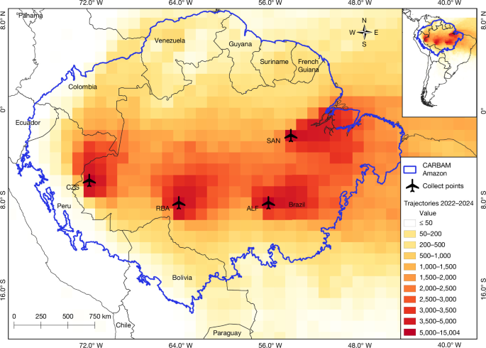
Here, we report CO2 and CO measurement results from the four Amazonian aircraft vertical profile sites of the CARBAM project38 (SAN: 2.86° S 54.95° W; ALF: 8.80° S 56.75° W; RBA: 9.38° S 67.62° W; in 2010–2012 for TAB: 5.96° S 70.06° W; and since 2013 for TEF: 3.39° S 65.60° W, and since 2022 for CZS: 7.00° S 72.50° W), detailed in refs. 1,13. The regions of influence for the four sites representing the northeast (SAN), southeast (ALF), southwest (RBA) and northwest Amazon region (TAB, 2010–2012; TEF, 2013–2021; CZS, 2022–2024) are shown in Extended Data Fig. 2c–h. Our samples were typically collected twice per month, totalling 1,017 vertical profiles over 15 years, in a descending spiral from 4,420 m to about 300 m a.s.l. In 2015, the vertical profile sampling was stopped in April at all sites and resumed in November at RBA. In 2016, vertical profiles were performed only at RBA and ALF. The vertical profiles were usually taken between 12:00 and 13:00 local time. Air samples were analysed by a non-dispersive infrared analyser for CO2 and by gas chromatography with HgO reduction detection for CO. The detailed analytical and sampling methods were presented in previous studies1,13.
Amazonia carbon study area
We defined the Amazonia study area according to subregions from ref. 39 and biomes from ref. 40, in which the studied area in Amazonia was determined to include only the forest ecosystems subregions: Amazonia stricto sensu, Guianas and Gurupi, with a total area of 6,700,798 km2.
Annual mean vertical profiles
The annual mean VP for each site was calculated by first producing the monthly mean for each height and then the annual mean for each height. The annual mean ∆VP for each site and for Amazonia was calculated by subtracting the corresponding background (BKG) for each VP and each height (Fig. 2 and Extended Data Fig. 3). To calculate the Amazonia annual mean VP, we applied the same method used to obtain the Amazonia annual mean flux and balance. To scale to the whole of Amazonia, we divided it into three regions (see ref. 13 and Supplementary Fig. 5). To compose the VP for region 1 (SAN + ALF), we calculated the weighted mean CO2 concentration at each height, proportional to the area of each region. To calculate the VP for region 2 (RBA + TAB, 2010–2012; RBA + TEF, 2013–2021; RBA + CZS, 2022–2024), the same procedure was used as in region 1. And for VP of region 3, the remaining Amazonia area not covered by the regions of influence of the vertical profile, we used the same VP as region 2. To compose the VP for Amazonia, the weighted mean for each height CO2 concentration was calculated, considering the three regions for each height (Supplementary Fig. 5).
Estimation of carbon fluxes
We used a column budget technique to estimate TCF, FCF and NBE, which consists of the difference between CO2 mole fraction measured in the vertical profile and the estimated background mole fraction41 (∆CO2), considering the travel time of air parcels along the trajectory from the coast to the site (equation (1)), following the methodology in refs. 1,13,42.
$${F}_{x}={\int }_{z=0(\mathrm{agl})}^{4.4\,\mathrm{km}(\mathrm{asl})}\frac{\Delta X}{t(z)}{\rm{d}}z.$$
(1)
Background
Background mole fractions were estimated according to the methodology described in ref. 41, using the geographical position of each air-mass back-trajectory from the HYSPLIT model43 when it intersects two virtual limits: (1) a latitude limit, from the Equator southwards at 30° W and (2) a line between two observation sites at Ragged Point, Barbados (RPB), and Ascension Island, the United Kingdom (ASC), from NOAA/GML. We used CO2 (ref. 44) and CO (ref. 45) concentrations from the NOAA/GML Carbon Cycle Cooperative Global Air Sampling Network to determine the background.
Carbon fire fluxes
We calculated fire emissions according to the methods published in refs. 1,13. We used observed CO/CO2 ratios by site from 2010 to 2024 (CO/CO2, ppb CO per ppm CO2) from measured CO mole fractions. The CO/CO2 ratios were calculated from clearly identifiable plumes in the vertical profiles during the dry season along period study (39 VP ALF CO/CO2 = 60.7 ± 30.7 ppb ppm−1; 35 VP SAN CO/CO2 = 56.1 ± 20.4 ppb ppm−1; 44 VP RBA CO/CO2 = 67.7 ± 24.1 ppb ppm−1; and 19 VP TTC (TAB_TEF_CZS) CO/CO2 = 74.2 ± 29.1 ppb ppm−1), which represents how many ppb CO is emitted for each 1 ppm CO2 during burning process. To calculate CO2 from fire, we used the CO flux and subtracted it from natural CO emissions (equation (2)). After the step \({F}_{\mathrm{CO}}-{F}_{\mathrm{CO}}^{\mathrm{Natu}{\rm{r}}\mathrm{al}}\), we used the CO/CO2 ratio to estimate the amount of CO2 from fire. NBE represents all processes from natural sources and sinks and all anthropogenic non-fire emissions (or after fire, without CO emissions) (NBE = total − fire).
$${{\rm{FC}}}_{{\rm{Fire}}}={R}_{{{\rm{CO}}}_{2}:{\rm{CO}}}({F}_{{\rm{CO}}}-{F}_{{\rm{CO}}}^{{\rm{Natural}}}).$$
(2)
Flux uncertainty analysis by Monte Carlo error propagation
Flux uncertainties were estimated using Monte Carlo error propagation (1,000 iterations). CO2 measurement uncertainty was 0.03 ppm, and background (BKG) uncertainties were derived from residuals to the fitted CO2 smooth curve, according to ref. 1. Uncertainties in back-trajectory travel times13 were also included. For carbon fire emissions and NBE, uncertainties in CO/CO2 ratios, CO fluxes and a 25% uncertainty in natural CO emissions were considered. VP flux uncertainties were derived from the Monte Carlo ensemble. Monthly uncertainties were estimated using pooled standard deviation to account for intra-month variability within the annual mean flux, and period uncertainties were calculated using the quadratic mean.
An additional source of uncertainty is the limitation on sampling to 4.4 km a.s.l. Transit times of air parcels from the coast to sampling sites, based on HYSPLIT, can vary, with mean trajectory times of 2.6 days for SAN, 5.3 days for ALF, 6.6 days for RBA, 5.7 days for TAB, 5.0 days for TEF and 7.6 days for CZS. The convective process, together with long travel times of air masses, can represent loss of carbon sources and sink contributions from the surface, because our vertical profiles start at 4.4 km. Comparing the background concentration and the top of vertical profiles is one way to verify potential information loss1,13. According to the method we use, the flux is obtained by subtracting the measured CO2 mole fraction in the VP from the background concentration, accounting for the integration time (equation (1)). During the dry season, the loss of information is larger to positive (VP > BKG), because during the burning season (peak of the dry season), the top of VP starts with a higher CO2 concentration than BKG due to convective processes driven by biomass burning.
A previous study46 proposed a correction of our gas concentration measurements based on a comparison of laboratory analyses of samples collected on 12 vertical profiling flights above Manaus in 2017–2019. The in situ measurements were made with a cavity ring-down spectrometer (CRDS), and discrete flask samples (PFPs) collected on the same flights were analysed in the laboratory. Some of the continuous CRDS measurements differed from those determined in the laboratory from flask samples (PFP) collected on the same flights (Figure A4 in ref. 46). Based on linear regression of N = 158 paired CRDS-PFP measurements, ref. 46 reported that water vapour content explained only 13% of the variance in the CRDS-PFP differences (Figure A7 in ref. 46). Nevertheless, ref. 46 proposed applying this regression relationship to adjust all laboratory measurements. Applying such an adjustment would conflate multiple methodological differences between the two sampling and analytical systems. The regression in ref. 46 compares independent instruments sampling distinct air parcels under different pressures, flow rates and materials. The proposed correction assumes that the in situ CRDS measurements are accurate, that the laboratory analyses are biased, that discrepancies arise solely from water vapour, and that the regression relationship can be extrapolated to approximately 13,319 laboratory measurements collected over 15 years. For these reasons, the proposed adjustment was not applied in this study. LaGEE measurements used in this study are internally consistent across the full temporal and spatial domain.
An additional source of uncertainty is addressed in the calculation of fire carbon emissions and NBE. Over time, the forest is becoming drier and hotter. These changes promote a lower CO/CO2 ratio. The use of a single mean CO/CO2 ratio is another source of uncertainty, leading to lower fire emissions than those observed in recent years because the ratio tends to decline over time. It is likely that carbon emissions from fires were higher than our averages for 2023 and 2024 indicate, because both were drought years.
Missing data imputation
We used the missForest algorithm to impute missing monthly TCF and FCF data at the ALF, SAN, RBA and TAB_TEF_CZS (TTC) sites. These gaps resulted from sampling and logistical issues in the laboratory. The missForest method is a non-parametric imputation approach based on random forests47,48, and we implemented it in R language49 through the missForest package50. To estimate missing values for TCF and FCF1,13, we included the following monthly variables in the imputation process: temperature (T), precipitation (P), vapour pressure deficit (VPD), ONI, TNA index, EVI, burned area (BA) and fire spots (FS). The missing data gaps were imputed using average values calculated from 1,000 runs of missForest. The normalized root mean square errors obtained for FCTotal and FCFire were 0.0014 and 0.0012 for ALF, 0.0011 and 0.0010 for RBA, 0.0055 and 0.0053 for SAN and 0.0018 and 0.0016 for TTC, respectively. NBE missing data were calculated by subtracting the fire from TCF.
Regions of influence
We define regions of influence as those areas covered by the density of back-trajectories51. We updated the calculations for the regions of influence used in our published CO2 papers1. In this study, the regions received two treatment steps. In the first step, we calculated back trajectories for altitudes lower than 1,300 m. As we have only four heights below 1,300 m, the density of trajectories could be reduced, compromising the representativeness. To better characterize atmospheric circulation over the quarters and years, we calculated trajectories at each sampling height (>1,300 m) twice a week, at the same locations and time of day, over the 15 years for each VP sampling site. A second treatment in the grid cells was done to increase the weight for the grid cells near the sample site. We normalized the weight for the region of influence to be from 0 to 1. First, the grid with a value of 1 was calculated by disregarding 2.5% of the grids with the highest values, thereby increasing the area of the grid region with a value of 1. It was considered a regular grid of 1° × 1° generated in the WGS 84 georeference system (EPSG:4326).
Precipitation, temperature, VPD and EVI data
We used the quarterly regions of influence maps as spatial weighting functions for all studied parameters to determine how each parameter influenced the carbon flux and for the missing data imputation process (missForest), following ref. 4. We used the GPCP database (http://eagle1.umd.edu/GPCP_ICDR/GPCP_Monthly.html), v.1.3, for precipitation analysis (described in refs. 52,53,54), which contains daily data at a 1° × 1° latitude–longitude resolution. We used 2-m temperatures from ERA-5 that are monthly means of daily means since 1959, and which were used with a resolution of 0.25° × 0.25° latitude–longitude, obtained from the European Centre for Medium-Range Weather Forecasts (ECMWF)27,55. The VPD product is a measure of the indirect vapour pressure deficit in kPa (resolution of 2.5 arcmin) of monthly means of temperature and humidity, provided by the Climatic Research Unit Ts4.0 (ref. 56). The dataset was resampled to a 1° × 1° spatial resolution using the monthly mean. The EVI is a vegetation index that aims to estimate the fraction of photosynthetically active radiation (fPAR) from terrestrial vegetation. The EVI product used57 was the MANVI: Moderate Resolution Imaging Spectroradiometer (MODIS) multiangle implementation of atmospheric correction nadir-solar (see the methods in ref. 13).
Burned area
Two products of burned area (BA) were used: (1) for all annual burned areas, the BA from MapBiomas was used, integrating all types of vegetation that were burned (primary and secondary forest, pasture, agriculture and others), from the MapBiomas Fire Collection 4 (ref. 25; https://brasil.mapbiomas.org). MapBiomas Fire was validated with a global accuracy of 89% (ref. 33); (2) for monthly BA (used only for missForest calculation), MODIS products were used: MODIS Collection 6 MCD64A1 burned area product13,58.
Deforestation
The procedures to retrieve deforestation as geographic data built by PRODES/INPE21 based on a historical series of Landsat images provide deforestation annual increments in the Brazilian Amazon. Detailed information on the PRODES methodology is available and can be accessed at http://urlib.net/rep/8JMKD3MGP3W34R/443H3RE (ref. 59). The dataset accuracy is 93.5 (ref. 60). We used the data period from 2010 to 2024. Using QGIS software, a 0.25° × 0.25° grid was generated for the entire Brazilian Amazon, which was filled with the absolute values of deforested area calculated for each cell and each year of the series. The mean deforestation area was calculated for the period 2010–2024 within each grid cell. Annual deforestation data correspond to the deforested area mapped by the PRODES project in a given year for Amazon forests.
Monthly deforestation and degradation
Monthly deforestation and degradation data correspond to either the deforestation alerts (clear cut, deforestation with vegetation, and mining) or degradation alerts (ordered selective logging, disordered selective logging, burns and degradation) captured by the DETER61 Amazon system in a given month. This dataset is produced daily by the visual interpretation of medium spatial resolution optical imagery of National Institute for Space Research (INPE) and, although not a full estimate of deforestation and degradation in the Amazon, can indicate variations in deforestation patterns over time33,62. We used the raw version of the dataset provided by INPE that included both password-protected data and data collected from August 2015.
Fire spots
Fire spots in Pan-Amazonia between 2010 and 2024 and burned area in Brazilian Amazon were retrieved from the BDQueimadas wildfire monitoring program of INPE63 (see the methods in ref. 13).
ONI
Warm (El Niño) and cold (La Niña) periods based on a threshold of ±0.5 °C for the ONI, 3-month running mean of ERSST v.5 SST anomalies in the Niño 3.4 region (5° N–5° S, 120° W–170° W), based on centred 30-year base periods updated every 5 years (ref. 26). To analyse the intensity of the events, we used the ONI classification anomaly28—for El Niño events, weak (0.5–0.9 °C), moderate (1.0–1.4 °C), strong (1.5–1.9 °C), and very strong (≥2.0 °C).
TNA index
The TNA index was computed as the mean sea-surface temperature (SST) anomaly over the region 23.5° N–5.5° N and 57.5° W–15° W (ref. 64). Monthly SST fields were obtained from ERA5 (0.25°), and anomalies were derived relative to a 30-year climatological baseline (1971–2000), consistent with standard TNA calculations27. We used the same ONI anomaly classification to analyse the intensity of the TNA warming events.
Statistical analysis
Annual data (2010–2024) for the Amazon included TCF, precipitation (P), temperature (T), ONI, TNA index, fire spots (FS), burned area (BA), annual deforestation (DEF) and accumulated deforestation (DEF_acc). Variable distributions and homogeneity of variance were assessed using the Shapiro–Wilk and Levene’s tests (Supplementary Table 1), respectively. Although most variables met normality assumptions, robust statistical approaches were adopted because of the small sample size (n = 15) and potential deviations from Gaussian behaviour typical of environmental datasets (Supplementary Discussion 3). Principal component analysis was applied to standardized data, with the first two components considered to represent the dominant variability. The k-means clustering (k = 3) was performed in the principal component analysis space, with cluster characteristics summarized in a standardized heatmap. The optimal number of clusters was determined using the average silhouette width (Extended Data Fig. 4).
Group differences among clusters were assessed using Welch’s analysis of variance (Supplementary Table 1), which is robust to heteroscedasticity and unequal sample sizes. When significant differences were detected (P < 0.05), pairwise comparisons were conducted using the Games–Howell post hoc test (Supplementary Table 1), which does not assume equal variances and appropriately controls the type I error rate under these conditions. This approach provides a consistent and reliable framework for identifying differences among clusters in environmental variables (Supplementary Discussion 2). All analyses were conducted in R language49.
Amazonia pasture, soybean and mining area
We obtained annual estimates of pasture, soybean cropland and mining area across Amazonia from the MapBiomas Collection 1024 dataset (30 m spatial resolution). Annual land-cover maps were used to isolate class-specific pixels (pasture, soybean and mining) and to compute their corresponding areas (km2) within the Amazonia carbon study area. This approach provided a consistent time series of land-use expansion and persistence for 2000–2024.
Lightning-associated wildfires
After 2017, in group 3, the years with accurate data were 2023 and 2024, when a more accurate cloud-to-ground lightning dataset was available. We used cloud-to-ground strokes from the Earth Networks Total Lightning Network (ENTLN)65. In South America, particularly in Amazonia, ENTLN lacks a dense sensor network comparable to that in other regions of Brazil. Even so, it operates with a stroke detection efficiency above 50% (corresponding to a flash detection efficiency above 80%) and a mean location accuracy below 1 km. Just for reference, in regions with high sensor densities, after the 2021 upgrade, the ENTLN reaches cloud-to-ground flash detection efficiency levels above 95% and median location accuracy below 100 m (ref. 66). Although performance depends on regional sensor coverage, ENTLN is considered one of the most advanced and reliable lightning networks globally67. Active fires used in this study were provided by the Visible Infrared Imaging Radiometer Suite on the Suomi National Polar-Orbiting Partnership satellite, with a spatial resolution of 375 m. The Visible Infrared Imaging Radiometer Suite 375 m active fire product provides geolocation accuracy of the order of one pixel (about 375 m), with typical sub-pixel geolocation uncertainties (about 70 m), ensuring reliable spatial representation of fire locations. All overpasses, day and night, were used from the Wildfire Monitoring Program of the INPE, available at http://www.inpe.br/queimadas/ (ref. 63). To assess lightning-associated wildfire among all cloud-to-ground lightning strokes, we identified probable lightning candidates that occurred up to 72 h (3 days) before active fire detection, using a fixed buffer radius of 1 km around each active fire and accounting for the location accuracy of both datasets. A detailed description of lightning candidate characteristics in Brazil is provided in ref. 68.