Bound states in the continuum through quantum interference in ultracold atomic collisions

Experimental details

We begin by preparing an ultracold two-component gas of 6Li atoms in the two lowest hyperfine states, namely, \(| a \rangle\) and \(| b \rangle\), confined in an optical dipole trap inside a steel vacuum chamber50. The trapped gas is then transported into a glass cell using a focus-tunable lens. Performing the experiment inside the glass cell is essential to achieve the required modulation depth of the oscillating magnetic field. A schematic of the experimental sequence is shown in Extended Data Fig. 1. After transfer, a short spectrally broadened rf pulse is applied to ensure an equal spin mixture of \(| a \rangle\) and \(| b \rangle\). The magnetic field is then ramped to 820 G, where a second dipole trap is switched on forming a crossed dipole trap, enabling efficient evaporative cooling. Evaporation is terminated just before molecule formation sets in, resulting in temperatures below 600 nK and estimated trap frequencies of {fx = 715 Hz, fy = 1,239 Hz, fz = 1,474 Hz}. The ultracold cloud is subsequently brought to the target magnetic field near 543 G, where it is held for 200 ms to allow the field to stabilize, resulting in the faint horizontal feature of the static I = 2 Feshbach resonance visible in Fig. 2b. The Floquet modulation is then applied for 100 ms, generated by two resonantly driven LC circuits26. After modulation, the magnetic field is ramped back to 763 G, and the remaining atoms are detected via the resonant absorption imaging of state \(| b \rangle\) on the D2 transition. Far from resonance, approximately 3,500 atoms remain after the full sequence of magnetic-field ramps and Floquet modulation. At a temperature of 600 nK and using the trap frequencies given above, this corresponds to a Fermi temperature of approximately 1.45 µK, resulting in T/TF ≈ 0.4.

To probe the elastic interaction strength, we perform trap-quench measurements, as described in ref. 26. The gas is prepared following the procedure above, except that evaporation is performed only in the transport trap, without the crossed-beam configuration. During the application of the Floquet drive, the trap power is suddenly reduced from 1 W to 200 mW, exciting collective breathing dynamics. After a variable evolution time, the Floquet drive is switched off and the cloud is imaged immediately.

For the rf photoassociation measurements, the sequence is slightly modified (Extended Data Fig. 2). After preparing an equal mixture of \(| a \rangle\) and \(| b \rangle\), the magnetic field is ramped to 600 G, where a Landau–Zener sweep transfers atoms from \(| b \rangle\) to \(| c \rangle\). The resulting \(| a \rangle\) –\(| c \rangle\) mixture is then evaporatively cooled at 300 G to below 600 nK, before the magnetic field is ramped to the target value of 544 G. After allowing the magnetic field to stabilize, a high-power σx-polarized rf pulse with a Rabi frequency of 2π × 81 kHz is applied for a duration of 400 ms to drive the photoassociation transition from the continuum of \(| a \rangle\)–\(| c \rangle\) scattering states to the \(| a \rangle\)–\(| b \rangle\) continuum. To observe the BIC, Floquet modulation polarized along the quantization axis is applied simultaneously. The remaining atoms are detected using the absorption imaging of state \(| c \rangle\).

We also evaluated the potential impact of sample heating on the rf photoassociation. A temperature increase translates to a spectroscopic frequency shift of \({\Delta }\nu =\frac{{\Delta }T{k}_{{\rm{B}}}}{h}\), which would manifest as a broadening of the photoassociation profiles. Because we do not detect any substantial distortion or broadening in our spectroscopic data, we conclude that the actual heating remains minimal. Furthermore, since the initial \(| a \rangle\)–\(| c \rangle\) mixture is prepared far from any scattering resonance, the short-range component of its wavefunction varies slowly with energy. The governing Franck–Condon factors are, therefore, minimally affected by heating.

The Floquet modulation depth Brf is calibrated via the a.c. Zeeman shift of the hyperfine levels induced by the drive, following the procedure in ref. 26.

Derivation of the effective Hamiltonian

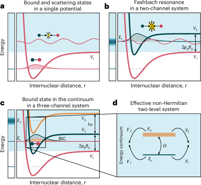
The effective non-Hermitian two-level Hamiltonian used to describe the avoided crossing of two Floquet–Feshbach resonances can be derived by using the Feshbach–Fano projection technique51. We consider two discrete molecular states \(| 1 \rangle\) and \(| 2 \rangle\) with bare energies E1 and E2, respectively, coherently coupled with strength Ω.

Since Floquet theory can be understood as the classical limit of quantized field theory26,52, both states are coupled to a set of Floquet continuum channels, labelled by index n. This index denotes scattering continua that differ by the number of drive quanta, such that the total number of drive quanta is given by N = N0 + n. Throughout the main text, we denote this quantity by ΔN; here we use n for brevity. The classical limit is then formally recovered as N0 → ∞. The total Hamiltonian consists of three contributions:

$$H={H}_{\rm{d}}+{H}_{\rm{c}}+V,$$

(3)

where

$${H}_{\rm{d}}={E}_{1}| 1 \rangle \langle 1| +{E}_{2}| 2 \rangle \langle 2| +\Omega \left(| 1 \rangle \langle 2| +| 2 \rangle \langle 1| \right)$$

(4)

describes the two discrete molecular states and their coherent coupling,

$${H}_{\rm{c}}=\sum _{n}\int\,dE\,E| E,n \rangle \langle E,n|$$

(5)

describes the Floquet continua and

$$V=\sum _{i=1,2}\sum _{n}\int\,dE\,\left[{W}_{in}(E)| i \rangle \langle E,n| +{W}_{in}^{* }(E)| E,n \rangle \langle i| \right],$$

(6)

accounts for the coupling between the molecular states and the continua. Here Win(E) denotes the coupling matrix element between the discrete state \(| i \rangle\) and the continuum state \(| E,n \rangle\).

Using the projectors onto the discrete and continuum subspaces51, we get

$$Q=| 1 \rangle \langle 1| +| 2 \rangle \langle 2| ,\qquad P=1-Q.$$

(7)

Applying these projectors to the stationary Schrödinger equation yields

$$\left(QHQ-E\right)Q| \varPsi \rangle +QHP\,P| \varPsi \rangle =0,$$

(8)

$$PHQ\,Q| \varPsi \rangle +\left(PHP-E\right)P| \varPsi \rangle =0.$$

(9)

Solving the second equation for the continuum component gives

$$P| \varPsi \rangle =\dfrac{1}{{E}^{+}-PHP}PHQ\,Q| \varPsi \rangle ,$$

(10)

where E+ = E + i0+ imposes outgoing-wave boundary conditions. Inserting this expression into the first equation gives an effective equation in the discrete subspace:

$${H}_{{\rm{eff}}}(E)Q| \varPsi \rangle =EQ| \varPsi \rangle ,$$

(11)

with

$${H}_{{\rm{eff}}}(E)=QHQ+QHP\dfrac{1}{{E}^{+}-PHP}PHQ.$$

(12)

Thus, the coupling to the continuum produces the self-energy

$$\varSigma (E)=QHP\dfrac{1}{{E}^{+}-PHP}PHQ.$$

(13)

In the basis \(\{| 1 \rangle ,| 2 \rangle \}\), the effective Hamiltonian becomes

$${H}_{{\rm{eff}}}(E)=\left(\begin{array}{cc}{E}_{1}&\Omega \\ \Omega &{E}_{2}\end{array}\right)+\left(\begin{array}{cc}{\varSigma }_{11}(E)&{\varSigma }_{12}(E)\\ {\varSigma }_{21}(E)&{\varSigma }_{22}(E)\end{array}\right).$$

(14)

Using the continuum representation introduced above, the self-energy matrix elements are

$${\varSigma }_{ij}(E)=\sum _{n}\int\,d{E}^{{\prime} }\dfrac{{W}_{in}({E}^{{\prime} }){W}_{jn}^{* }({E}^{{\prime} })}{{E}^{+}-{E}^{{\prime} }}.$$

(15)

With the identity53,

$$\dfrac{1}{{E}^{+}-{E}^{{\prime} }}={\mathcal{P}}\dfrac{1}{E-{E}^{{\prime} }}-i\uppi \delta (E-{E}^{{\prime} }),$$

(16)

the self-energy separates into a real dispersive shift and an imaginary decay:

$${{\varSigma }}_{ij}(E)={{\Delta }}_{ij}(E)-\frac{{\rm{i}}}{2}{{\varGamma }}_{ij}(E),$$

(17)

where

$${\Delta }_{ij}(E)=\sum _{n} \mathcal P \int \,{\rm{d}}{E}^{{\prime} }\frac{{W}_{in}({E}^{^{\prime} }){W}_{jn}^{* }({E}^{^{\prime} })}{E-{E}^{^{\prime} }},$$

(18)

and

$${\varGamma }_{ij}(E)=2\uppi \sum _{n}{W}_{in}(E){W}_{jn}^{* }(E).$$

(19)

The terms Δ11 and Δ22 shift the resonance energies, whereas the off-diagonal terms Δ12 and Δ21 modify the coupling. In the following, these shifts are absorbed into the definitions of E1, E2 and Ω.

To obtain the minimal model, we assume that the coupling matrix elements are approximately energy independent over the narrow energy window relevant to the avoided crossing:

$${W}_{in}(E)\simeq {w}_{i}^{(n)}.$$

(20)

Equation (19) then becomes

$${\varGamma }_{ij}=2\uppi \sum _{n}{w}_{i}^{(n)}{w}_{j}^{(n)* }.$$

(21)

Defining the partial decay rate of state \(| i \rangle\) into continuum n as

$${\gamma }_{i}^{(n)}=2\uppi {\left\vert {w}_{i}^{(n)}\right\vert }^{2},$$

(22)

one obtains

$${\varGamma }_{ii}=\sum _{n}{\gamma }_{i}^{(n)}$$

(23)

for the diagonal elements. The off-diagonal elements are

$${\varGamma }_{12}=\sum _{n}\sqrt{{\gamma }_{1}^{(n)}{\gamma }_{2}^{(n)}}{e}^{i{\phi }_{n}},$$

(24)

where \({\phi }_{n}=\arg {w}_{1}^{(n)}-\arg {w}_{2}^{(n)}\) is the relative phase with which the two discrete states couple to continuum n. If the relevant couplings can be chosen real, this reduces to

$${\varGamma }_{12}={\varGamma }_{21}=\sum _{n}\sqrt{{\gamma }_{1}^{(n)}{\gamma }_{2}^{(n)}}.$$

(25)

The resulting non-Hermitian effective Hamiltonian is, therefore,

$${H}_{\mathrm{eff}}=\left(\begin{array}{cc}{E}_{1} & {\Omega }\\ {\Omega } & {E}_{2}\end{array}\right)-\frac{{\rm{i}}}{2}\sum _{n}\left(\begin{array}{cc}{\gamma }_{1}^{(n)} & \sqrt{{\gamma }_{1}^{(n)}{\gamma }_{2}^{(n)}}\\ \sqrt{{\gamma }_{1}^{(n)}{\gamma }_{2}^{(n)}} & {\gamma }_{2}^{(n)}\end{array}\right).$$

(26)

This expression generalizes the usual non-Hermitian effective Hamiltonian3,24,38 of the Friedrich–Wintgen BIC mechanism to the case of several Floquet continua. Each continuum channel contributes to the individual decay rates of the two discrete states through the diagonal terms. At the same time, any continuum also generates an off-diagonal, continuum-mediated coupling.

The entrance channel corresponds to the Floquet continuum with n = 0. Further simplifications follow from the structure of the Floquet channels. Because the energy of a single drive quantum (hν) far exceeds the kinetic energy scale (kBT) considered here, all channels with n > 0 are energetically closed.

Furthermore, inelastic loss is dominated by single-photon processes. We, therefore, retain only the two relevant continua, that is, n = 0 and n = − 1. Equation (26) then reduces to

$${H}_{\mathrm{eff}}=\left(\begin{array}{cc}{E}_{1} & {\Omega }\\ {\Omega } & {E}_{2}\end{array}\right)-\frac{{\rm{i}}}{2}\left(\begin{array}{cc}{\gamma }_{1}+{\gamma }_{1}^{{\prime} } & \sqrt{{\gamma }_{1}{\gamma }_{2}}+\sqrt{{\gamma }_{1}^{{\prime} }{\gamma }_{2}^{{\prime} }}\\ \sqrt{{\gamma }_{1}{\gamma }_{2}}+\sqrt{{\gamma }_{1}^{{\prime} }{\gamma }_{2}^{{\prime} }} & {\gamma }_{2}+{\gamma }_{2}^{{\prime} }\end{array}\right).$$

(27)

Here we have defined

$${\gamma }_{i}^{(0)}\equiv {\gamma }_{i},\qquad {\gamma }_{i}^{(-1)}\equiv {\gamma }_{i}^{{\prime} }.$$

(28)

The unprimed rates, thus, describe coupling to the entrance channel continuum, whereas the primed rates describe coupling to the n = − 1 Floquet continuum.

The BIC condition (equation (2)) follows from minimizing the decay width of one of the eigenstates of Heff. Since the imaginary parts of the eigenvalues determine the resonance widths, the BIC occurs when one width becomes minimal and the other, maximal. Solving this condition with respect to the detuning δ = E1 − E2 yields equation (2).

Parameter dependence of the BIC

The position of the BIC is not fixed by a single control parameter, but depends on the combined tuning of the static magnetic field, Floquet drive and collision energy. To map this dependence and to identify suitable parameters for the rf photoassociation measurements, we performed coupled-channel calculations for different modulation frequencies ν and collision energies Ekin above the \(| a \rangle\)–\(| b \rangle\) dissociation threshold at a modulation strength of Brf = 6.5 G.

For each modulation frequency, we calculated the inelastic scattering cross-section as a function of the magnetic field and collision energy, and identified the BIC from the disappearance of the resonant loss feature associated with the avoided crossing. This yields both magnetic field BBIC and energy EBIC at which the BIC condition is fulfiled (Extended Data Fig. 3). Below the dissociation threshold, the numerically calculated molecular bound state energy is shown.

Over the frequency range considered here, both quantities vary linearly with the modulation frequency. This shows that the Floquet modulation frequency provides direct control over both magnetic-field position and collision energy of the BIC. In particular, it allows us to move the BIC from the dissociation threshold deeper into the scattering continuum and to choose parameters for which it can be probed by rf photoassociation spectroscopy. Supplementary Video 1 provides an animation showing the continuous evolution of the BIC as a function of modulation frequency.

An additional important observation from Extended Data Fig. 3a is that the suppression of coupling to the continuum persists over an energy range on the order of kB × 10 µK. This width is larger than the thermal energy spread of the atomic cloud, enabling the BIC to be resolved in loss spectroscopy measurements despite the finite temperature of the gas.

Coupled-channel calculations

At ultracold temperatures, two-body collisions are dominated by s-wave scattering and can be characterized by the complex s-wave scattering length as. For purely elastic collisions, as is real, whereas inelastic processes introduce an imaginary component that accounts for loss. The elastic and inelastic scattering cross-sections follow directly from as (ref. 54).

To compute as, we use coupled-channel methods, which are well-suited for cold atom systems in which multiple internal channels contribute to the scattering process. These methods solve the full multichannel Schrödinger equation, either in its differential form or, equivalently, as a set of coupled Lippmann–Schwinger integral equations. We solve the coupled Lippmann–Schwinger equations with an algorithm that expands the scattering wavefunction in Chebyshev polynomials to obtain accurate and numerically stable results55,56,57.

Accurate coupled-channel calculations require precise molecular interaction potentials. The potentials used in this work are based on high-resolution spectroscopic data58,59 and were further refined following the procedure of ref. 60. Details of the Floquet Hamiltonian used for the numerical results presented here are given in ref. 26. For the calculation of Im(as) relevant to the rf photoassociation data shown in Fig. 5d, we extend the Hamiltonian to include an additional field term that accounts for the σx-polarized rf spectroscopy drive.

For the thermally averaged inelastic cross-section shown in Fig. 2c, we compute σinel(Ec) for several collision energies Ec and perform a Boltzmann-weighted average. With p(Ec) as the Boltzmann distribution, the averaged cross-section is

$${\sigma }_{{\rm{inel}}}^{{\rm{avg}}}=\int\,p({E}_{\rm{c}}){\sigma }_{{\rm{inel}}}({E}_{\rm{c}}){\rm{d}}{E}_{\rm{c}}\,.$$

(29)

Because the magnetic resonance position depends on the collision energy, thermal averaging leads to an effective broadening of the resonances. The corresponding shift is given by \(\Delta B=\frac{{k}_{\rm{B}}\Delta T}{2{\mu }_{\rm{B}}}\), which amounts to 7.44 mG μK−1. For the cloud temperatures T < 600 nK used in the loss spectroscopy measurements, this leads only to a small broadening.

Parameters of the two-level Hamiltonian

To adapt equation (1) for modelling the avoided crossing between the (I = 2, ΔN = 0) and (I = 0, ΔN = + 1) Floquet–Feshbach resonances, the bare levels E1 and E2 must be redefined. We assign E2 to the static (I = 2, ΔN = 0) resonance, which is not Floquet dressed and, therefore, independent of the modulation frequency. Its energy is given by \({E}_{2}={\mu }_{\rm{B}}{B}_{{{I = 2}}}^{(0)}\), where \({B}_{{{I = 2}}}^{(0)}\) denotes the magnetic-field position of the conventional static I = 2 Feshbach resonance and μB denotes the Bohr magneton. By contrast, the (I = 0, ΔN = + 1) resonance assigned to E1 depends on the driving frequency ν. Although this dependence is generally nonlinear26, it can be well approximated as linear within the experimentally relevant frequency range. Accordingly, we model it as \({E}_{1}={\mu }_{\rm{B}}[{B}_{{{I = 2}}}^{(0)}+\kappa (\nu -{\nu }_{0})]\), where ν0 is the modulation frequency at which the two Floquet–Feshbach resonances would intersect at \({B}_{{{I = 2}}}^{(0)}\) in the absence of coupling Ω. With these definitions, the Hamiltonian in equation (1) becomes

$${H}_{\mathrm{eff}}=\left(\begin{array}{cc}{\mu }_{\rm{B}}[{B}_{\mathrm{I=2}}^{(0)}+\kappa (\nu -{\nu }_{0})] & {\Omega }\\ {\Omega } & {\mu }_{\rm{B}}{B}_{\mathrm{I=2}}^{(0)}\end{array}\right)-\frac{{{I}}}{2}\left(\begin{array}{cc}{\gamma }_{1}+{\gamma }_{1}^{{\prime} } & \sqrt{{\gamma }_{1}{\gamma }_{2}}+\sqrt{{\gamma }_{1}^{{\prime} }{\gamma }_{2}^{{\prime} }}\\ \sqrt{{\gamma }_{1}{\gamma }_{2}}+\sqrt{{\gamma }_{1}^{{\prime} }{\gamma }_{2}^{{\prime} }} & {\gamma }_{2}+{\gamma }_{2}^{{\prime} }\end{array}\right)$$

(30)

from whose complex eigenvalues λ1/2 the magnetic resonance positions and widths are obtained via division by μB.

The parameters of equation (30) were determined through an iterative fitting procedure. First, the real part of the Hamiltonian was optimized so that Re(λ1/2) reproduced the experimentally observed resonance positions. Next, the imaginary part was adjusted to match Im(λ1/2) to the numerically calculated resonance widths. Because modifying the imaginary part slightly shifts the resonance positions, both steps were alternated until convergence was achieved. The resulting optimized parameters are listed in Extended Data Table 1.

Fitting of loss spectroscopic data

To fit the experimental loss data, we use a sum of Fano profiles61

$${N}_{{\rm{rel}}}(B)=\sum _{i}{N}_{i}\dfrac{{({q}_{i}+{\beta }_{i})}^{2}}{1+{\beta }_{i}^{2}}+{N}_{0}\,,$$

(31)

with the shape parameter q and

$${\beta }_{i}=\frac{B-{B}_{i}^{(0)}}{{\Delta }_{{i}}/2}\,,$$

(32)

where \({B}_{i}^{(0)}\) corresponds to the position and Δi is the width of the ith resonance. The factor N0 accounts for a constant offset and Ni scales the height of individual resonances.

From the loss spectroscopic data, the magnetic splitting \({\varDelta }_{{\rm{B}}}=({B}_{1}^{(0)}-{B}_{2}^{(0)})\) was extracted and from this, the coupling strength was calculated via 2Ω = μBΔB to obtain Fig. 2d.

Fitting of quench response

To quantify the elastic scattering contribution shown in Fig. 3a,b, we analyse the cloud’s response to a sudden trap quench following the procedure of ref. 26. At each evolution time, several absorption images were recorded and averaged, and the transverse density profile was fitted with a Gaussian to extract the cloud width σ(t). The resulting time series was then modelled by

$$\sigma (t)={\sigma }_{0}+A{e}^{-\gamma t}\cos \left(\omega t+\theta \right)+B{e}^{-{\gamma }_{\rm{B}}t},$$

(33)

where σ0 denotes the equilibrium width in the absence of oscillations. The oscillatory term describes the breathing-mode response of the trapped gas with amplitude A, damping rate γ, frequency ω and phase θ. The final exponential captures non-oscillatory relaxation processes with amplitude B and decay rate γB. Plotting A/γ reveals the elastic resonance response.