Pressure anisotropy-driven instabilities regulate the jovian magnetodisk

Magnetodisk crossings

Magnetodisk crossings are characterized by reversals in the measured magnetic field. For example, Supplementary Fig. 1 shows Juno’s observations during the crossing on August 30, 2017. One can see the direction of the magnetic field reverses at about 08:55 UT, indicating that Juno encountered the magnetodisk around this time. Based on these reversal signatures, ref. 31 identified 404 crossings in the radial extent from 20 to 100 RJ from the first 25 orbits of Juno. In this paper, we simultaneously analyze heavy ion pressure anisotropy and magnetic fluctuations during these crossings, as well as their relationship with plasma microscopic instabilities, which were not addressed in ref. 31 or in our subsequent studies45,46.

The orientation of the magnetodisk during a specific crossing can be derived from a minimum variance analysis (MVA)31 of the measured magnetic field. This analysis determines the directions along which the magnetic field changes most and least. In the case of the magnetodisk (which is a current sheet by nature), the former (L-axis) gives the direction of the magnetic field in the lobe regions, while the latter (N-axis) represents the normal to the magnetodisk. The third axis (M-axis) is along the cross-product of the N and L unit vectors and is approximately parallel to the current density in the magnetodisk31,45. Supplementary Fig. 1e–g shows the magnetic field in this local current sheet coordinate system for the crossing on August 30, 2017. As expected, the N component maintains a relatively steady, negative value, the M component oscillates around zero with a small amplitude, and the L component reverses directions during the crossing. This observation applies to all crossings identified by ref. 31. For further analysis, we define the component of the magnetic field normal to the magnetodisk (\({B}_{N}\)) by averaging the N component over a one-hour interval centered on the crossing time. The magnetic field in the lobe region (\({B}_{L}\)) is derived from a fit of the L component to a Harris current sheet model: \({B}_{L}=\tan \left[\left(t-{t}_{0}\right)/T\right]\), where \(t\) represents time, \({t}_{0}\) denotes the crossing time, and \({B}_{L}\) and \(T\) are free parameters.

Heavy ion plasma pressures

Figure 3 of ref. 46 shows that the cross-calibration between the JADE and JEDI datasets, including electrons, protons, and heavy ions, is statistically reliable. For electrons and protons, fluxes in the overlapping energy channels of the two instruments are in agreement, with no jump observed. Although there is no direct energy overlap between JADE and JEDI for heavy ions, the fluxes at the last three energy channels of JADE and the first three energy channels of JEDI (which can often be extended to a larger energy range; see Fig. 3c ref. 46) can be well fitted to a single power law, indicating consistency between the two instruments. These observations also hold for individual events. For instance, Supplementary Fig. 2 presents measurements from two example periods with evidence for dipolarization events, demonstrating the consistency between the JADE and JEDI datasets.

Therefore, we do not perform any further processing but simply combine the JADE and JEDI datasets to generate the number flux (\(J\)) sorted by energy (\(W\), from about 10 eV/e to 10 MeV/e) and pitch angle (\(\alpha\), ranging from \({0}^{\circ }\) to \({180}^{\circ }\)). Specifically, for heavy ions, we use the JAD-5-CALIBRATED-V1.0/SPECIES-5 and JED/NONPTOFXER/CDR/OXYGEN + SULFUR data from NASA’s Planetary Plasma Interactions (PDS). We then compute the number density (\(N\)), perpendicular pressure (\({P}_{\perp }\)) and parallel pressure (\({P}_{\parallel }\)) following the numerical integration method developed in ref. 46:

$$N=\sqrt{{2\pi }^{2}m}\int {W}^{-\frac{1}{2}}{{{\rm{d}}}}W\int \sin \alpha {{{\rm{d}}}}\alpha \cdot J\left(W,\alpha \right)$$

(1)

$${P}_{\perp }=\sqrt{2{\pi }^{2}m}\int {W}^{-\frac{1}{2}}{{{\rm{d}}}}W\int \sin \alpha {{{\rm{d}}}}\alpha \cdot J\left(W,\alpha \right)W{\sin }^{2}\alpha -\frac{1}{2}{Nm}{V}_{\perp }^{2}$$

(2)

$${P}_{{{{\rm{||}}}}}=\sqrt{8{\pi }^{2}m}\int {W}^{-\frac{1}{2}}{{{\rm{d}}}}W\int \sin \alpha {{{\rm{d}}}}\alpha \cdot J\left(W,\alpha \right)W{\cos }^{2}\alpha -{Nm}{V}_{{{{\rm{||}}}}}^{2}$$

(3)

where \({V}_{\perp }\) and \({V}_{\parallel }\) denote the perpendicular and parallel bulk velocities. Here, the parallel and perpendicular directions are defined with respect to the local magnetic field detected by MAG. We note that even at the magnetodisk center, the magnetic field remains well above the noisy level due to the present of a nonzero normal component across the entire magnetodisk31. Hence, the parallel and perpendicular directions, as well as the corresponding observables, can be reliably determined. In the calculation, we assume a mean mass (\(m\)) of 24 amu and a mean charge of 1.5 e, which corresponds to a composition of singly charged oxygen (O+) and doubly charged sulfur (S++) of equal number density and is close to observations29,30. Previous studies do indicate the existence of other ion species (e.g., O++, S+ and S+++) in the considered mass-charge ratio range. Nevertheless, their abundances are minor and do not significantly affect the mean mass and derived quantities (see Supplementary Note 3 for an estimate of their influence).

A preliminary examination indicates that the velocities of heavy ions derived from numerical integration might suffer from large errors. In addition, numerical velocity calculation may not be reliable for both protons and heavy ions off the center of the magnetodisk, where counts are generally low. Fortunately, refs. 45,46 shows the torque balance model provides a reasonable estimate of \({V}_{\perp }\). This model indicates that the electrodynamic torque exerted by the \(J\times B\) force associated with radial electric current balances the net transport of angular momentum carried by radial mass transport. That is,

$$\dot{M}\frac{d}{{dr}}\left(r{V}_{\perp }\right)=2\pi {r}^{2}{I}_{r}{B}_{n}$$

(4)

where \({I}_{r}\) represents radial electric current, \({B}_{n}\) represents the magnetic field component normal to the magnetodisk, and \(\dot{M}\) denotes the radial mass transport rate. Refs. 45,46 shows \({V}_{\perp }\) derived from Eq. 4, with \({I}_{r}\) from ref. 45 and \({B}_{n}\) from ref. 31 (both taken from Juno statistics) and \(\dot{M}=1500\) kg/s, fits ion velocities derived from JADE data using a forward modeling method30 well. Therefore, \({V}_{\perp }\) obtained in this way is used in Eq. 2 Additionally, we set \({V}_{\parallel }=0\) in Eq. 3 as Juno observations suggest that the field-aligned velocity component is negligible in general47.

Magnetic fluctuations

We first apply a high-pass filter (period\( < 150\) s) to the observed magnetic field to remove variations associated with the motion of Juno relative to the magnetodisk (e.g., magnetodisk crossings and flapping motion). Then, a Fast Fourier transformation is employed to calculate the power spectral density of the filtered magnetic field. By integrating the results over 6.7 mHz (corresponding to 150 s) to 4 Hz, we obtain the integrated power of magnetic fluctuations. The square root of this value gives the absolute amplitude (\({B}_{w}\)) of magnetic fluctuations analyzed in the main text.

Instability thresholds

Recent theoretical studies have highlighted the role of nonlinear effects, particularly at large wave amplitudes, in governing the growth and saturation of pressure anisotropy-driven instabilities20,21,24. These nonlinear processes influence not only the saturated fluctuation amplitudes and spectral features but also the timescales and relaxation pathways by which unstable plasmas evolve toward marginal stability. As an example of the latter, numerical simulations20 have shown that pressure anisotropy is regulated by particle scattering off smaller-scale fluctuations in the nonlinear firehose instability and by a balance between particle trapping within magnetic mirrors and scattering at the mirrors’ edges in the nonlinear mirror instability. These nonlinear mechanisms may determine the observed fluctuation amplitudes within the unstable regimes of the \(A\)-\({\beta }_{\parallel }\) space, as well as the formation of fine structures in particle VDFs.

The primary objective of this study, however, is to evaluate observationally whether the pressure anisotropy and magnetic fluctuations of Jupiter’s magnetodisk are organized by pressure anisotropy-driven instabilities in parameter space. To this end, we ignore the effects of nonlinear dynamics, following previous work on the solar wind15,16. Instead, we apply thresholds based on linear instability growth rates, which provide a first-order approximation of the boundaries delineating unstable regions in phase space. This approach facilitates direct comparison with Juno’s statistical measurements and is supported by the agreement between theoretical predictions and observational results (Figs. 1 and 2).

More specifically, to determine the thresholds of the mirror, cyclotron and firehose instabilities, we consider a plasma consisting of Maxwellian electrons (density \({N}_{e}\) and temperature \({T}_{e}\)), Maxwellian protons (density \({N}_{p}\) and temperature \({T}_{p}\)) and bi-Maxwellian heavy ions (density \({N}_{h}\), parallel temperature \({T}_{h\parallel }\) and perpendicular temperature \({T}_{h\perp }\)). In this context, \(A={T}_{h\perp }/{T}_{h\parallel }\). The parameters are taken from the statistical study44 at a radial distance of 50 RJ obtained by Juno: \({N}_{p}=0.32{N}_{h}\), \({N}_{e}=1.32{N}_{h}\), \({T}_{p}=8.5\) keV, \({T}_{e}=2.3\) keV, \({T}_{h\perp }=17.3\) keV and \({P}_{B}=8.2\times {10}^{-3}\) nPa. We calculated the maximum growth rate (\(\gamma\)) of the three instabilities in the region \(0.1 < {\beta }_{\parallel } < 100\) and \(0.1 < A < 5\) using the dispersion relation solver Waves in Homogeneous Anisotropic Magnetized Plasma (WHAMP)48. The relation \(\gamma={10}^{-3}{\omega }_{{cp}}\) (proton gyro-frequency) is then fitted for the three instabilities in the following equation15,16:

$${A}_{i}=1+\frac{{a}_{i}}{{\beta }_{\parallel }^{{b}_{i}}}$$

(5)

where \(i=m,c,f\) for the mirror, cyclotron and firehose instabilities, and \({a}_{i}\) and \({b}_{i}\) are the fitted parameters. The fitting results are (\({a}_{m}=\)1.03, \({b}_{m}=\)0.48), (\({a}_{c}=\)0.81, \({b}_{c}=\)0.32), and (\({a}_{f}=-\)0.52, \({b}_{f}=\)0.36). Strictly speaking, these fitted parameters are not constant and depend on parameters like \({T}_{e}\) and \({T}_{p}\), which vary at radial distances. Nevertheless, testing indicates that the fitting results are not sensitive to parameter variations within the range of Juno statistics. For example, using parameters at 80 RJ, where \({P}_{B}\) and \({T}_{h\perp }\) are 56% and 123% of those at 50 RJ, respectively, the threshold for the firehose instability becomes (\({a}_{f}=-\)0.56, \({b}_{f}=\)0.36). These values are very close to those obtained with parameters at 50 RJ; when plotted on the \(A\)-\({\beta }_{\parallel }\) plane, the two curves are nearly indistinguishable. Similar behavior is observed for the cyclotron and mirror instabilities as well.

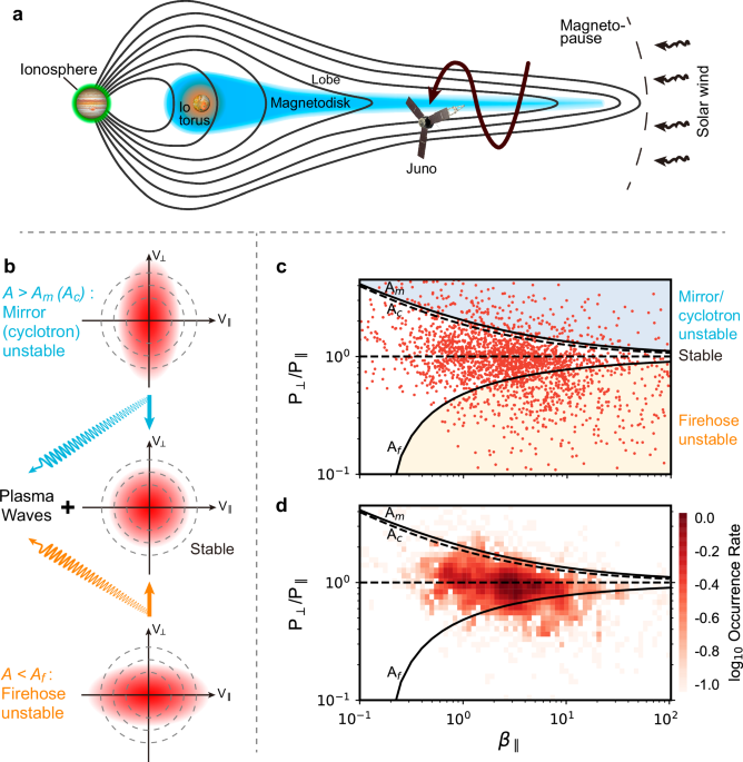
Both the mirror and cyclotron instabilities arise in the A > 1 regime. These two modes exhibit markedly different characteristics, particularly in terms of phase speed: The mirror mode is non-propagating, while the cyclotron mode propagates through the plasma with a finite phase speed. Consequently, they resonate with particles of different energies, which in turn affects both the time scale and pathway of the relaxation of unstable plasmas. However, from the perspective of linear instability theory, their instability thresholds are nearly identical, as shown, e.g., in Fig. 1c. Therefore, in this study, we address the two instability modes at the same time when comparing theoretical instability thresholds with observations.

Background dataset

To investigate the effects of magnetic dipolarization, we compare events with evidence for dipolarization events (data points circled by the red dashed contour in Fig. 3a) with the background. Previous studies have shown that plasma pressure and magnetic pressure depend on the positions where the observations are made. To eliminate the effects of this dependence, we construct a background dataset with the same spatial distributions as events with evidence for dipolarization events using the following method. First, we determine the spatial distribution of dipolarization events (the green-yellow coded contours in Fig. 3b). Then, we define the background dataset as the data points that meet two criteria: (1) they are located within the 0.1-level contour of the dipolarization event distribution shown in Figs. 3b and (2) they reside within the stable region depicted in Fig. 1c.