
5 days of this Machine Learning “Advent Calendar”, we explored 5 models (or algorithms) that are all based on distances (local Euclidean distance, or global Mahalanobis distance).
So it is time to change the approach, right? We will come back to the notion of distance later.
For today, we will see something totally different: Decision Trees!
 Decision Tree Regressor in Excel – image by author
Introduction with a Simple dataset
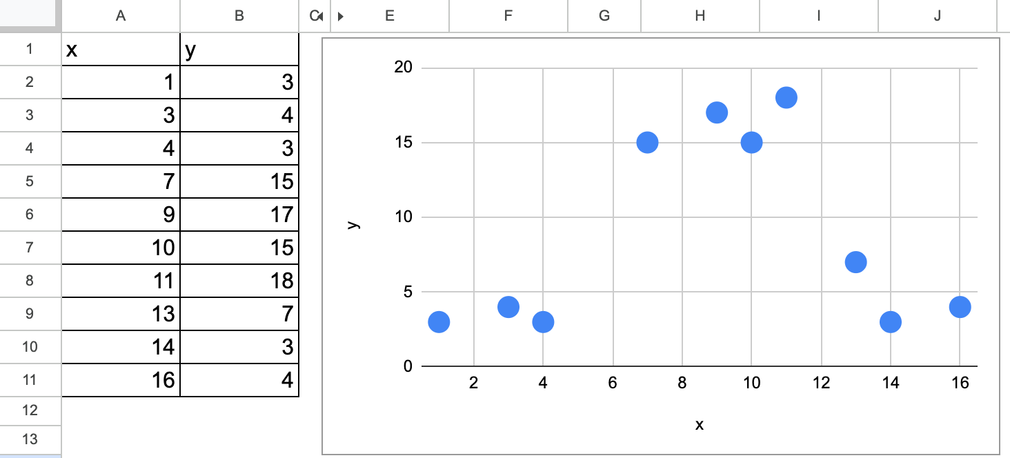
Let’s use a simple dataset with only one continuous feature.
As always, the idea is that you can visualize the results yourself. Then you have to think how to make the computer do it.
 Decision tree regression in Excel simple dataset (I generated myself) — image by author
We can visually guess that for the first split, there are two possible values, one around 5.5 and the other around 12.
Now the question is, which one do we choose?
This is exactly what we are going to find out: how do we determine the value for the first split with an implementation in Excel?
Once we determine the value for the first split, we can apply the same process for the following splits.
That is why we will only implement the first split in Excel.
The Algorithmic Principle of Decision Tree Regressors
I wrote an article to always distinguish three steps of machine learning to learn it effectively, and let’s apply the principle to Decision Tree Regressors.
So for the first time, we have a “true” machine learning model, with non-trivial steps for all three.
What is the model?
The model here is a set of rules, to partition the dataset, and for each partition, we are going to assign a value. Which one? The average value y of all the observations in the same group.
So whereas k-NN predicts with the average value of the nearest neighbors (similar observations in terms of features variables), the Decision Tree regressor predicts with the average value of a group of observations (similar in terms of the feature variable).
Model fitting or training process
For a decision tree, we also call this process fully growing a tree. In the case of a Decision Tree Regressor, the leaves will contain only one observation, with thus a MSE of zero.
Growing a tree consists of recursively partitioning the input data into smaller and smaller chunks or regions. For each region, a prediction can be calculated.
In the case of regression, the prediction is the average of the target variable for the region.
At each step of the building process, the algorithm selects the feature and the split value that maximizes the one criterion, and in the case of a regressor, it is often the Mean Squared Error (MSE) between the actual value and the prediction.
Model Tuning or Pruning
For a decision tree, the general term of model tuning is also call it pruning, be it can be seen as dropping nodes and leaves from a fully grown tree.
It is also equivalent to say that the building process stops when a criterion is met, such as a maximum depth or a minimum number of samples in each leaf node. And these are the hyperparameters that can be optimized with the tuning process.
Inferencing process
Once the decision tree regressor is built, it can be used to predict the target variable for new input instances by applying the rules and traversing the tree from the root node to a leaf node that corresponds to the input’s feature values.
The predicted target value for the input instance is then the mean of the target values of the training samples that fall into the same leaf node.
Split with One Continuous Feature
Here are the steps we will follow:
List all possible splits
For each split, we will calculate the MSE (Mean Squared Error)
We will select the split that minimizes the MSE as the optimal next split
All possible splits
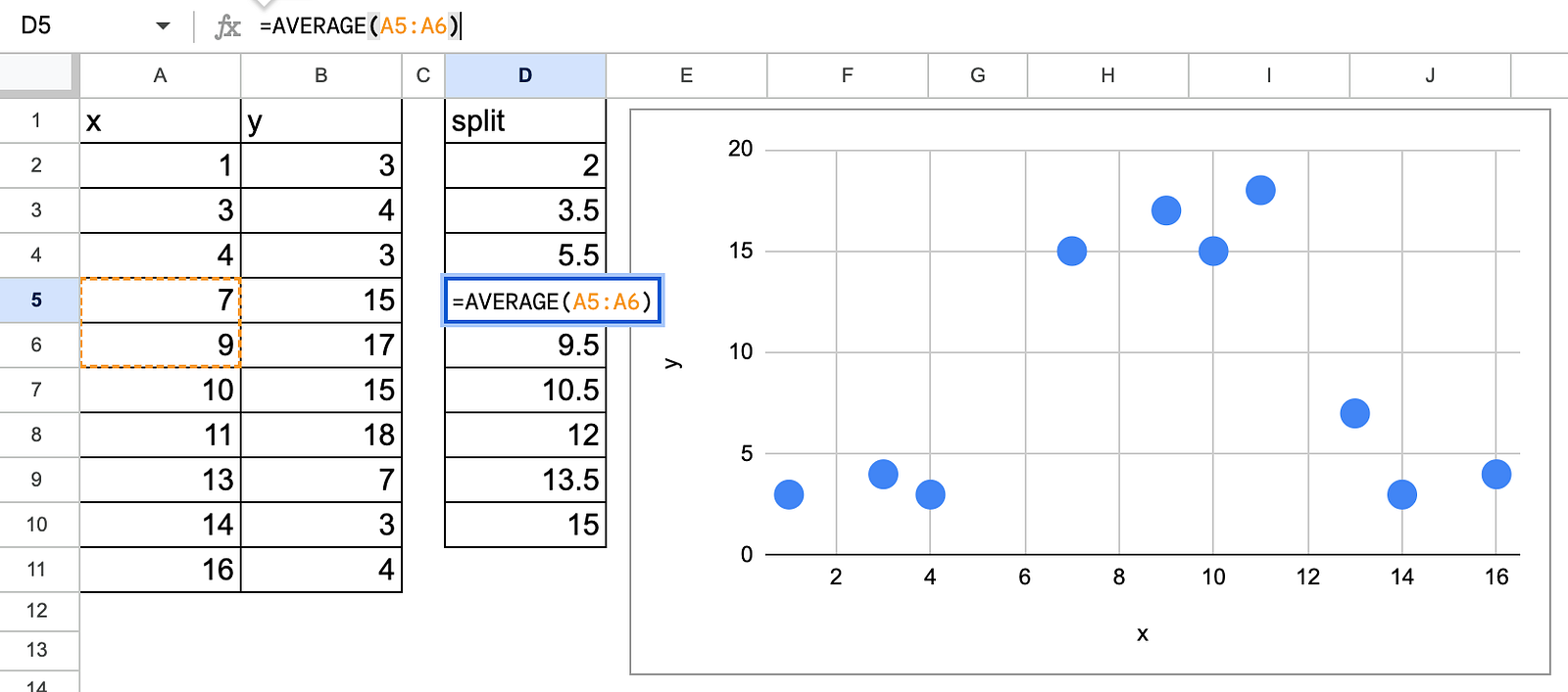
First, we have to list all the possible splits that are the average values of two consecutive values. There is no need to test more values.
 Decision tree regression in Excel with possible splits — image by author
MSE calculation for each possible split
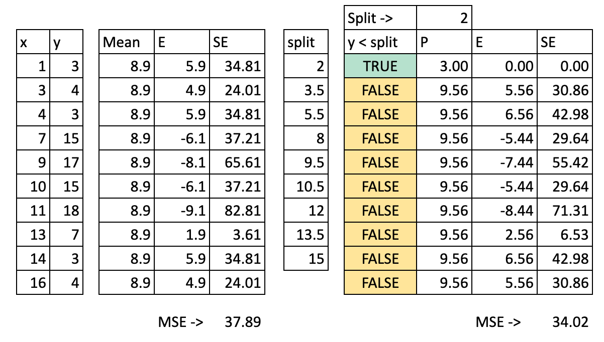
As a starting point, we can calculate the MSE before any splits. This also means that the prediction is just the average value of y. And the MSE is equivalent to the Standard Deviation of y.
Now, the idea is to find a split so that the MSE with a split is lower than before. It is possible that the split does not significantly improve the performance (or lower the MSE), then the final tree would be trivial, that is the average value of y.
For each possible split, we can then calculate the MSE (Mean Squared Error). The image below shows the calculation for the first possible split, which is x = 2.
 Decision tree regression in Excel MSE for all possible splits — image by author
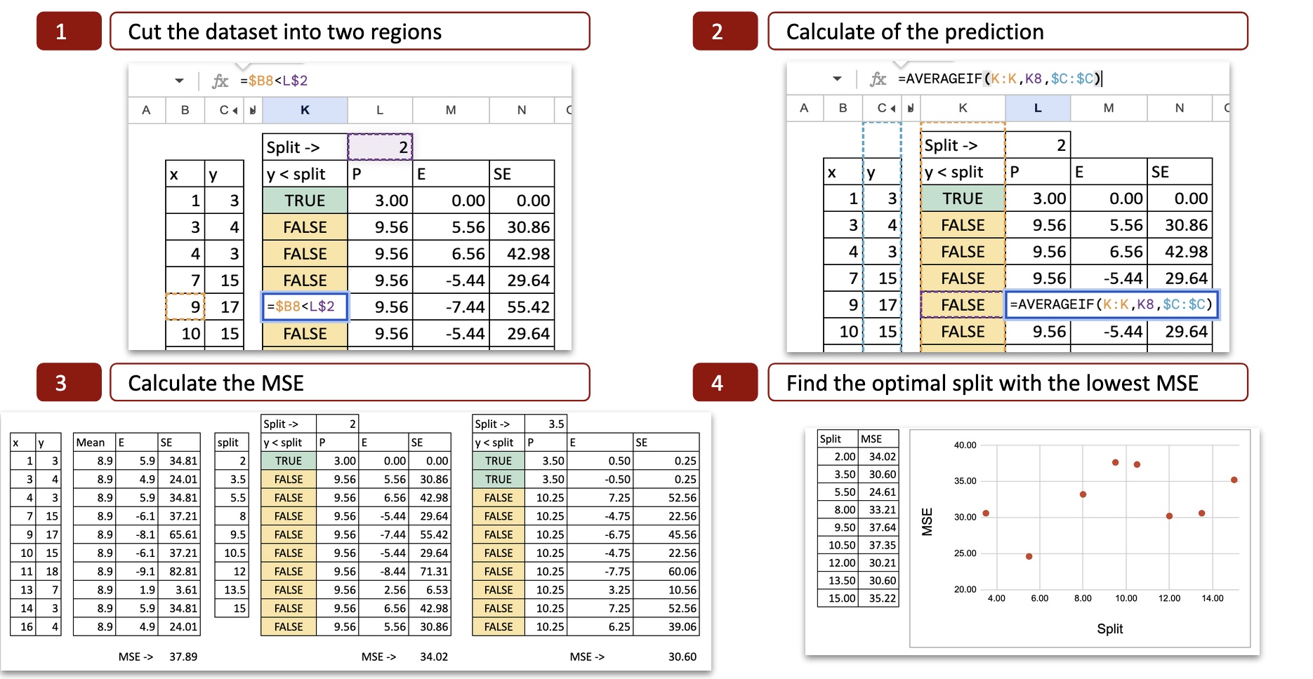
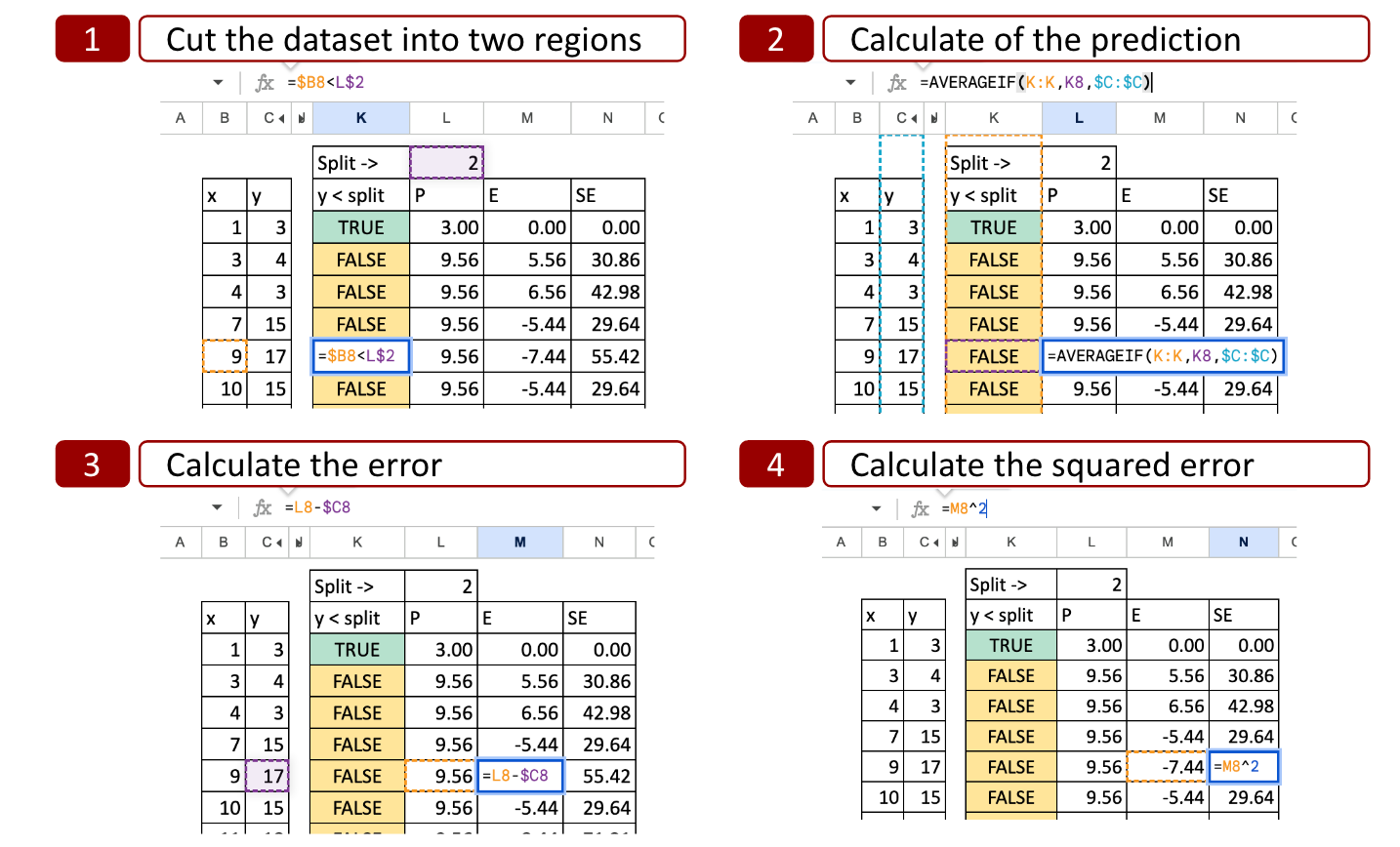
We can see the details of the calculation:
Cut the dataset into two regions: with the value x=2, we determine two possibilities x<2 or x>2, so the x axis is cut into two parts.
Calculate the prediction: for each part, we calculate the average of y. That is the potential prediction for y.
Calculate the error: then we compare the prediction to the actual value of y
Calculate the squared error: for each observation, we can calculate the square error.
 Decision tree regression in Excel with all possible splits — image by author
Optimal split
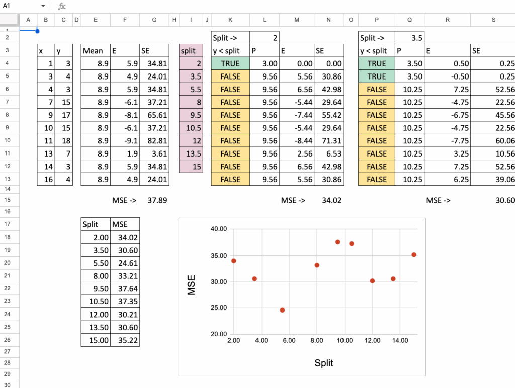
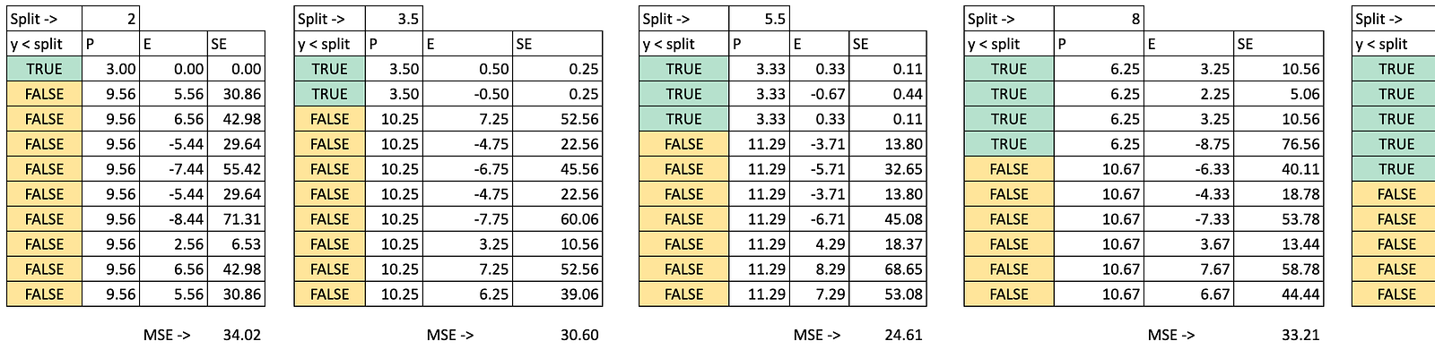
For each possible split, we do the same to obtain the MSE. In Excel, we can copy and paste the formula and the only value that changes is the possible split value for x.
 Decision tree regression in Excel splits— image by author
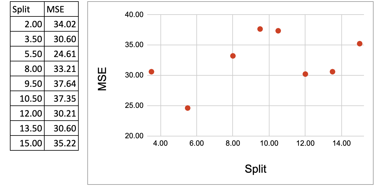
Then we can plot the MSE on the y-axis and the possible split on the x-axis, and now we can see that there is a minimum of MSE for x=5.5, this is exactly the result obtained with python code.
 Decision tree regression in Excel Minimumization of MSE — image by author
Now, one small exercise you can do is change the MSE to MAE (Mean Absolute Error).
And you can try to answer this question: what is the impact of this change?
Condensing All Split Calculations into One Summary Table
In the earlier sections, we computed each split step by step, so that we can better visualize the details of calculations.
Now we put everything together in one single table, so the whole process becomes compact and easy to automate.
To do this, we first simplify the calculations.
In a node, the prediction is the average, so the MSE is exactly the variance. And for the variance, we can also use the simplified formula:

So in the following table, we use one row for each possible split.
For each split, we calculate the MSE of the left node and the MSE of the right node.
The variance of each group can be simplified using the intermediate results of y and y squared.
Then we compute the weighted average of the two MSE values. And in the end, we get exactly the same result as in the step-by-step method.
 Decision Tree Regressor in Excel – get it from here – image by author
Split with Multiple Continuous Features
Now we will use two features.
This is where it becomes interesting.
We will have candidate splits coming from both features.
How do we choose?
We will simply consider all of them, and then select the split with the smallest MSE.
The idea in Excel is:
first, put all possible splits from the two features into one single column,
then, for each of these splits, calculate the MSE like before,
finally, pick the best one.
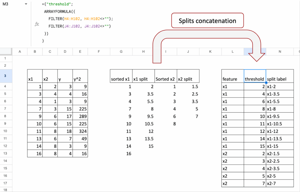
Splits concatenation
First, we list all possible splits for Feature 1 (for example, all thresholds between two sorted values).
Then, we list all possible splits for Feature 2 in the same way.
In Excel, we concatenate these two lists into one column of candidate splits.
So each row in this column represents:
“If I cut here, using this feature, what happens to the MSE?”
This gives us one unified list of all splits from both features.
 Decision Tree Regressor in Excel – get it from here – image by author
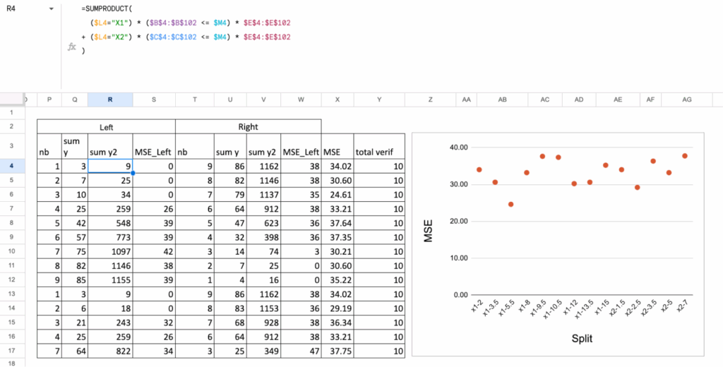
MSE calculations
Once we have the list of all splits, the rest is the same logic as before.
For each row (that is, for each split):
we divide the points into left node and right node,
we compute the MSE of the left node,
we compute the MSE of the right node,
we take the weighted average of the two MSE values.
At the end, we look at this column of “Total MSE” and we choose the split (and therefore the feature and threshold) that gives the minimum value.
 Decision Tree Regressor in Excel – get it from here – image by author
Split with One Continuous and One Categorical Feature
Now let us combine two very different types of features:
one continuous feature
one categorical feature (for example, A, B, C).
A decision tree can split on both, but the way we generate candidate splits is not the same.
With a continuous feature, we test thresholds.
With a categorical feature, we test groups of categories.
So the idea is exactly the same as before:
we consider all possible splits from both features, then we select the one with the smallest MSE.
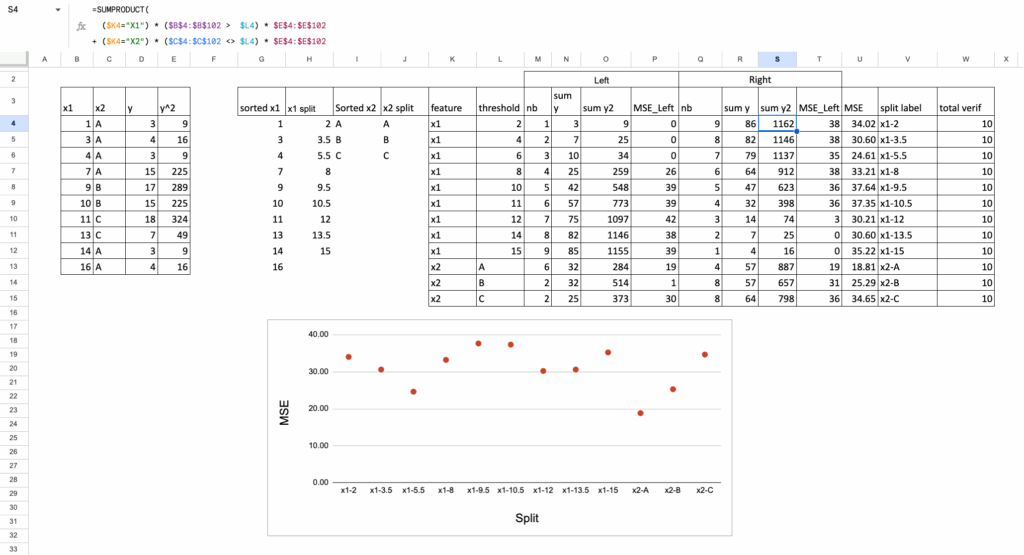
Categorical feature splits
For a categorical feature, the logic is different:
each category is already a “group”,
so the simplest split is: one category vs all the others.
For example, if the categories are A, B, and C:
split 1: A vs (B, C)
split 2: B vs (A, C)
split 3: C vs (A, B)
This already gives meaningful candidate splits and keeps the Excel formulas manageable.
Each of these category-based splits is added to the same list that contains the continuous thresholds.
MSE calculation
Once all splits are listed (continuous thresholds + categorical partitions), the calculations follow the same steps:
assign each point to the left or right node,
compute the MSE of the left node,
compute the MSE of the right node,
compute the weighted average.
The split with the lowest total MSE becomes the optimal first split.
 Decision Tree Regressor in Excel – get it from here – image by author
Exercise you can try out
Now, you can play with the Google Sheet:
You can try to find the next split
You can change the criterion, instead of MSE, you can use absolute error, Poisson or friedman_mse as indicated in the documentation of DecisionTreeRegressor
You can change the target variable to a binary variable, normally, this becomes a classification task, but 0 or 1 are also numbers so the criterion MSE still can be applied. But if you want to create a proper classifier, you have to apply the usual criterion Entroy or Gini. It is for the next article.
Conclusion
Using Excel, it is possible to implement one split to gain more insights into how Decision Tree Regressors work. Even though we didn’t create a full tree, it is still interesting, since the most important part is finding the optimal split among all possible splits.
One more thing about missing values
Have you noticed something interesting about how features are handled between distance-based models, and decision trees?
For distance-based models, everything must be numeric. Continuous features stay continuous, and categorical features must be transformed into numbers. The model compares points in space, so everything has to live on a numeric axis.
Decision Trees do the inverse: they cut features into groups. A continuous feature becomes intervals. A categorical feature stays categorical.
And a missing value? It simply becomes another category. There is no need to impute first. The tree can naturally handle it by sending all “missing” values to one branch, just like any other group.