
QiankunNet with transformer architecture
In the study of quantum systems, we encounter complex structures characterized by N interacting components, each represented by discrete quantum variables \(\left\vert {{{\bf{x}}}}\right\rangle=\{{x}_{1},{x}_{2},…{x}_{N}\}\). These variables might represent various physical quantities such as spin state or particle occupation numbers. The challenge lies in describing the many-body wave function, which establishes a sophisticated mapping between the configuration space and a vast landscape of complex numbers.
$$\left\vert \Psi \right\rangle=\sum\limits_{{{{\bf{x}}}}}\left\langle \right.{{{\bf{x}}}}\left\vert \Psi \right\rangle \left\vert {{{\bf{x}}}}\right\rangle=\sum\limits_{{{{\bf{x}}}}}\Psi ({{{\bf{x}}}})\left\vert {{{\bf{x}}}}\right\rangle$$
(4)
where each configuration is represented by an occupation number vector \(\left\vert {{{\bf{x}}}}\right\rangle=\{{x}_{1},{x}_{2},…,{x}_{N}\}\), with xi ∈ {0, 1} indicating whether the i-th spin orbital is occupied or not. This mapping encodes both magnitude and phase information of the quantum state, essentially serving as a transformation engine that converts a given many-body configuration x into its corresponding quantum mechanical description Ψ(x). By leveraging artificial neural networks, we aim to construct an efficient approximation of the wave function’s behavior. This neural network approach effectively creates a trainable computational framework that learns to replicate the wave function’s response to different input configurations. Among the various neural architectures available in modern machine learning, we focus our investigation on the Transformer framework, particularly in its application to quantum many-body systems. The Transformer architecture implements a sophisticated attention-based structure: an embedding layer that maps the physical configurations into a high-dimensional representation space, followed by multiple self-attention layers that capture the intricate correlations between quantum variables. The architecture is particularly well-suited for quantum systems due to its ability to model long-range interactions and complex quantum correlations through its multi-head attention mechanism. The connection between NLP and quantum chemistry represents a substantive interdisciplinary bridge rather than a superficial analogy. By establishing a formal mathematical isomorphism between configuration strings in quantum systems and sentences in language models, we address the shared challenge of exponential complexity that has long hindered progress in both fields. Specifically, the Hilbert space dimension of 2N for N spin orbitals parallels the exponential growth of possible sentences in natural language, creating a compelling theoretical foundation for methodological transfer. In our implementation, Transformer architectures represent quantum wave functions with quantum bitstrings serving as inputs to predict the wave function. Particularly noteworthy is how the autoregressive property of Transformers enables efficient modeling of conditional probabilities in quantum states, mirroring their function in language prediction.
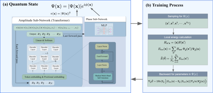
Our QiankunNet consists of two complementary sub-networks: the amplitude sub-network and the phase sub-network. This dual-network architecture effectively captures both the magnitude and phase information necessary to fully describe a quantum state:
$$\Psi ({{{\bf{x}}}})=| \Psi ({{{\bf{x}}}})| {e}^{i\phi ({{{\bf{x}}}})},$$
(5)
where the amplitude sub-network is constructed using a Transformer decoder to represent the probability ∣Ψ(x)∣2, while the phase sub-network ϕ(x) employs a multi-layer perceptron (MLP) as shown in Fig. 1a. The Transformer architecture1,5 is built from layers, each containing a self-attention component composed of multiple independent attention heads. These heads operate in parallel, each with its own set of parameters, allowing the network to simultaneously learn different types of correlations. Within each head, the attention mechanism works by computing how relevant each input position is to every other position, creating a rich network of relationships within the quantum state configuration. The processing of quantum states through our Transformer network follows a carefully designed sequence of steps. The initial state of the decoder is calculated using the input token vector and the position embedding matrix. We prepare the input by adding a special marker (a zero bit) at the beginning of the binary configuration. This augmented input then undergoes an embedding process, where each binary value is transformed into a rich, high-dimensional representation that captures the quantum mechanical properties of the system. The network takes as input a token/qubit vector x = {x1, x2, . . . , xn} of length n, which is transformed into embeddings:
$$P{E}^{(0)}=[e({x}_{1}),e({x}_{2}),\ldots,e({x}_{n})]+P\in {{\mathbb{R}}}^{n\times {d}_{{{{\rm{model}}}}}}$$
(6)
where e(xi) represents the dmodel-dimensional learnable embedding of token xi, P is the matrix of learnable position embeddings, and PE(0) contains the combined embeddings for the input sequence at the initial layer. Position information plays a crucial role in quantum states, so we incorporate learned positional encodings for each site in the configuration. These encodings help the network understand the spatial relationships between different components of the quantum system. The embedded and position-encoded information then flows through multiple identical Transformer layers. Each layer in our architecture processes the quantum state information through several stages. The masked multi-head attention mechanism allows the network to learn complex correlations while maintaining the autoregressive property—ensuring that each position only influences those that come after it. For each decoder layer l = 1, 2, …, L, the following operations are performed: The masked multi-head self-attention mechanism computes:
$${{{{\rm{Attention}}}}}^{(l)}(Q,K,V)={{{\rm{softmax}}}}\left(\frac{Q{K}^{T}}{\sqrt{{d}_{k}}}+M\right)V$$
(7)
where \(Q=P{E}^{(l-1)}{W}_{Q}^{(l)}\), \(K=P{E}^{(l-1)}{W}_{K}^{(l)}\), and \(V=P{E}^{(l-1)}{W}_{V}^{(l)}\) are the queries, keys, and values linearly transformed from the positionally encoded embeddings PE(l−1), M is the mask ensuring autoregressive property, and dk is the dimension of the keys. Residual connections and layer normalization are applied:
$${H}^{(l)}=P{E}^{(l-1)}+{{{{\rm{Sublayer}}}}}^{(l)}\left({{{\rm{LayerNorm}}}}(P{E}^{(l-1)})\right)\in {{\mathbb{R}}}^{n\times {d}_{{{{\rm{model}}}}}}$$
(8)
where Sublayer(l)(PE(l−1)) represents the output of the masked multi-head self-attention sublayer for layer l. Position-wise feed-forward networks with GeLU activation function process the information:
$${{{{\rm{FFN}}}}}^{(l)}(H)={{{\rm{GeLU}}}}({H}^{(l)}{W}_{1}^{(l)}+{b}_{1}^{(l)}){W}_{2}^{(l)}+{b}_{2}^{(l)}\in {{\mathbb{R}}}^{n\times {d}_{{{{\rm{model}}}}}}$$
(9)
where \({W}_{1}^{(l)}\in {{\mathbb{R}}}^{{d}_{{{{\rm{model}}}}}\times {d}_{{{{\rm{ff}}}}}}\) and \({W}_{2}^{(l)}\in {{\mathbb{R}}}^{{d}_{{{{\rm{ff}}}}}\times {d}_{{{{\rm{model}}}}}}\) are weight matrices, \({b}_{1}^{(l)}\in {{\mathbb{R}}}^{{d}_{{{{\rm{ff}}}}}}\) and \({b}_{2}^{(l)}\in {{\mathbb{R}}}^{{d}_{{{{\rm{model}}}}}}\) are bias vectors, and GeLU is the Gaussian Error Linear Unit activation function. The output for the next layer is set as:
$$P{E}^{(l)}=\left({H}^{(l)}+{{{{\rm{FFN}}}}}^{(l)}({{{\rm{LayerNorm}}}}({H}^{(l)}))\right)\in {{\mathbb{R}}}^{n\times {d}_{{{{\rm{model}}}}}}$$
(10)
which serves as input to the next layer or as the final output if l = L. After processing through L layers, the Transformer decoder’s final output undergoes linear transformation and softmax activation to produce the conditional probability distribution:
$$P({x}_{n}| {x}_{1},{x}_{2},\ldots,{x}_{n-1})={{{\rm{softmax}}}}(P{E}^{(L)}{W}_{{{{\rm{out}}}}})\in {{\mathbb{R}}}^{n\times {d}_{{{{\rm{out}}}}}}$$
(11)
where \({W}_{{{{\rm{out}}}}}\in {{\mathbb{R}}}^{{d}_{{{{\rm{model}}}}}\times {d}_{{{{\rm{out}}}}}}\) is the projection weight matrix for the output layer, and dout is the dimension of the output space. The probability of a sequence x = (x1, x2, …, xn) can be factorized as a product of conditional probabilities:
$$P(x)=P({x}_{1},{x}_{2},\ldots,{x}_{n})={\prod }_{i=1}^{n}P({x}_{i}| {x}_{1},{x}_{2},\ldots,{x}_{i-1})$$
(12)
expressing the joint probability P(x) of the sequence as the product of conditional probabilities of each element xi given its preceding elements. The complex probability amplitude Ψ(x) for sequence x is defined as:
$$\Psi (x)=\sqrt{P(x)}{e}^{i\phi (x)}=| \Psi ({{{\bf{x}}}})| {e}^{i\phi ({{{\bf{x}}}})}$$
(13)
Here, Ψ(x) combines the square root of probability P(x) with a complex phase factor eiϕ(x). The phase ϕ(x) is represented by a Multi-Layer Perceptron network that processes the input sequence x and outputs a real-valued phase, effectively encoding the complex quantum correlations present in the electronic wavefunction.
Efficient sampling strategy
Monte Carlo sampling is used to generate samples {x1, x2, …, xN} for quantum states. A common choice is a Markov-chain Monte Carlo (MCMC) black-box sampler. MCMC is a class of algorithms based on Markov chains for random sample generation, where the production of each state depends only on the previous state. A classic example of MCMC is the Metropolis-Hastings algorithm, which uses an acceptance-rejection mechanism to decide whether to move to a new state.
$${p}_{{{{\rm{accept}}}}}=\min (1,p({{{{\bf{x}}}}}^{{\prime} })/p({{{\bf{x}}}})).$$
(14)
It can be seen that a Markov chain that gradually approximates the target distribution \({p}_{\overrightarrow{\theta }}({{{\bf{x}}}})\) is constructed, so that the distribution of states on the chain eventually matches the target distribution. However, MCMC involves the sequential assessment of proposed configurations, while the computational cost increases in relation to both the desired quality of the sample collection and the overall quantity of samples. With a Metropolis sampling scheme, Choo et al.32 observed that the performance was highly dependent on the number of samples used, but this was constrained to a maximum batch size of Ns = 106. For VMC-based quantum chemistry, a more efficient scheme called autoregressive sampling can be introduced, which generates independent, uncorrelated samples directly from the target distribution. Rather than trying to model the distribution over every possible configuration of these discrete variables simultaneously, autoregressive sampling builds the distribution sequentially. It takes advantage of the fact that the probability of a specific configuration can be decomposed into the product of conditional probabilities. This approach allows for sampling one variable at a time, given the values of the previously sampled variables, thus reducing the complexity and computational burden significantly. Autoregressive sampling algorithm generates probability distributions p(x) of the special form
$$p({{{\bf{x}}}})=p({{{{\bf{x}}}}}_{1},{{{{\bf{x}}}}}_{2},\ldots,{{{{\bf{x}}}}}_{N})={\prod }_{i}^{N}p({{{{\bf{x}}}}}_{i}| {{{{\bf{x}}}}}_{ < i})$$
(15)
The autoregressive sampling scheme allows for the generation of exact samples without the need for a pre-thermalization step or the discarding of intermediate samples (which is necessary in Monte Carlo (MC) sampling to avoid autocorrelations). This makes autoregressive neural networks generally more efficient than MC sampling. As illustrated in Fig. 5, the generation of a single quantum state configuration uses QiankunNet’s sequential autoregressive sampling scheme. The architecture shows how each orbital’s occupation probability is computed conditionally based on previously sampled orbitals through the Transformer decoder layers. The probability distribution of the quantum states can be efficiently sampled by leveraging the factorization property ∣Ψ(x)∣2 = ∣Ψ(x1)∣2∣Ψ(x2∣x1)∣2∣Ψ(x3∣x1, x2)∣2 ⋯ ∣Ψ(xN∣x1, …, xN−1)∣2 and the masked attention mechanism that ensures the network output at position n only depends on positions m<n. We implement the sampling procedure by generating one bit at a time: we first compute ∣Ψ(x1)∣2 and sample the first bit x1, then using the sampled x1, we compute ∣Ψ(x2∣x1)∣2 and sample x2, followed by computing ∣Ψ(x3∣x1, x2)∣2 and sampling x3 using all previous bits, and so on until all N bits have been sampled. This sequential sampling strategy is essential for the VMC optimization of our neural quantum states, as it enables simultaneous sampling and network training: while generating configurations for energy estimation, the network parameters can be updated through gradient computation, effectively integrating the sampling and optimization processes into a unified workflow.
Fig. 5: Generation of a single quantum state configuration using QiankunNet’s sequential autoregressive sampling scheme.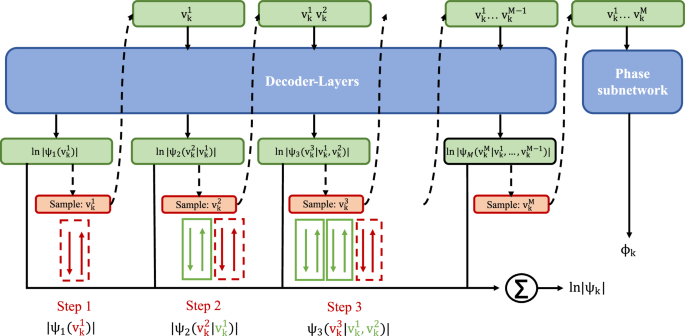
This approach consists of decoder layers that process sequential conditional probabilities, where each step computes the conditional probability of a quantum variable vk given its previous variables. The network includes a phase subnetwork that computes the phase ϕk, and all components contribute to the final wave function ∣ψk∣. The dashed arrows indicate the autoregressive sampling process, where each variable is sampled conditionally on previously generated variables. Green boxes represent input tokens \({v}_{k}^{i}\) at different positions in the sequence. Blue boxes denote the Transformer decoder layers and phase subnetwork components. Orange boxes show the sampling operations at each step. Red dashed boxes highlight the newly sampled variables at each step, while green solid boxes indicate previously sampled variables that serve as context for subsequent sampling. The summation symbol (∑) represents the aggregation of all contributions to compute the final wave function amplitude.
Moreover, our training employs a dynamic sample adjustment mechanism that monitors the number of unique quantum states generated during sampling and automatically adjusts the total sample size accordingly. Through this adaptive approach, the sampling process naturally adjusts to the complexity of different molecular systems and the convergence state of the model, ensuring efficient training without manual tuning of sampling parameters for each specific case. The sampling process naturally forms a Monte Carlo quaternary tree structure, where each layer corresponds to a spatial orbital. While our model represents each spin–orbital as a binary token (0 or 1), the MCTS algorithm groups spin-orbitals by spatial orbital for efficiency. Since each spatial orbital contains two spin-orbitals (spin-up and spin-down), this yields four possible combined states at each tree node: “00”, “01”, “10”, or “11”. This grouping reduces the tree depth from 2N to N levels for a system with N spatial orbitals, effectively building up the complete electronic configuration through a hierarchical sampling process. Figure 6 illustrates our batched autoregressive sampling implementation. Fig. 6a presents the algorithm for generating a single configuration, showing how orbital occupations are sampled sequentially with electron number constraints. Fig. 6b depicts the tree structure used for batch generation, where multiple samples are generated simultaneously using a combination of breadth-first search (BFS) for the first few orbitals followed by depth-first search (DFS) for the remaining orbitals. This hybrid approach balances exploration diversity with memory efficiency. In the initial phase, the system explores the first few orbital positions using BFS, assigning probability weights to possible orbital configurations. This ensures reasonable coverage of the sampling space, avoiding premature convergence to local optima. Subsequently, the system shifts to a DFS strategy for processing the remaining orbital positions, a key design primarily aimed at optimizing computational resources, especially memory usage. Through this depth-first approach, the system only needs to retain state information of the current sampling path in memory, rather than simultaneously storing complete states of all possible paths, significantly reducing memory requirements, as shown in Algorithm 2 within Supplementary Information. This memory-efficient design enables the model to handle larger-scale quantum systems without being strictly limited by hardware resources. This hybrid sampling strategy is not only more efficient in computational resource utilization but also maintains sampling diversity while guiding the sample distribution to converge to the minimum energy quantum state configuration, accurately characterizing the ground state properties of quantum many-body systems. A key feature of our MCTS sampling implementation is the incorporation of physical constraints through efficient pruning strategies. Since the total number of electrons Ne is conserved in quantum chemical systems, we can significantly reduce the sampling space by eliminating invalid branches of the sampling tree. This pruning mechanism ensures that we only sample physically meaningful configurations while significantly reducing the computational cost. This tree-like structure of our sampling procedure bears resemblance to the MCTS used in AlphaGo50, but with a crucial distinction: while AlphaGo’s MCTS relies on extensive backtracking to explore the game tree and evaluate different strategies, our method employs pure forward autoregressive sampling without any backtracking. This fundamental difference arises from the distinct nature of quantum state sampling, where our goal is to efficiently generate physically valid electronic configurations that follow the wave function probability distribution, rather than exploring multiple strategic paths as in game-playing scenarios. The absence of backtracking in our approach not only simplifies the sampling process but also significantly enhances its computational efficiency while maintaining the ability to capture the quantum state’s probability distribution accurately. This sampling strategy enables the simultaneous generation of multiple configuration samples, dramatically improving the efficiency of quantum Monte Carlo calculations. By generating independent samples directly, we eliminate both the correlation issues inherent in MCMC methods and the computational overhead of backtracking processes, while also enabling more accurate estimation of physical observables through larger sample batches. In Fig. 7, we showcase a comparison between the performance of MCMC sampling and the MCTS method for H2O system. From this comparison, it becomes evident that the computational time of the MCMC method increases as the number of samples grows, and the low acceptance probability associated with the Metropolis-Hastings algorithm renders it inefficient for larger sample sizes. In contrast, the computational time of the MCTS method exhibits a nearly constant behavior, since it is primarily dependent on the number of unique samples. A computational efficiency improvement of several orders of magnitude is achieved compared to the MCMC method. Figure 7b illustrates that, with the same number of samples (e.g., 105), the MCTS method achieves chemical accuracy within 1500 steps, whereas the MCMC method fails to attain chemical accuracy even after an extensive number of steps.
Fig. 6: Illustration of the Monte-Carlo tree search (MCTS) autoregressive sampling process which represented as a Monte-Carlo quaternary tree structure.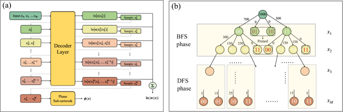
a The autoregressive sampling (AS) algorithm generates one sample per run. Each node in (b) corresponds to a particular local sampling outcome, and the number on the edge pointing to each circle indicates the weight. Ns can be chosen to be any number (Ns = 1000 is used as an example). Each node has four possible states (unoccupied, spin-up, spin-down, or doubly occupied). The sampling proceeds layer by layer, with each layer corresponding to one orbital’s occupation state. This sampling strategy combines Breadth-First Search (BFS) and Depth-First Search (DFS) approaches. The tree is naturally pruned based on electron number conservation: branches that would lead to configurations with incorrect total electron numbers are eliminated (shown in gray dashed lines). This pruning significantly reduces the sampling space and ensures that only physically valid configurations are generated.
Fig. 7: Comparison between different sampling algorithms.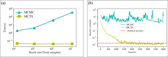
a The time comparison of H2O system for Markov Chain Monte Carlo (MCMC) and Monte-Carlo tree search (MCTS) autoregressive sampling methods. In both cases, the QiankunNet is used for the wave function ansatz. b The convergence comparison of H2O between MCMC and MCTS sampling methods. Ns = 105 is used as an example, where Ns denotes the number of samples used in the variational Monte Carlo calculation for estimating the energy expectation value.
Variational Monte Carlo optimization
The VMC algorithm then proceeds iteratively to optimize QiankunNet using energy as the loss function, as illustrated in Fig. 1b: at each step, we sample configurations from the current wave function ∣Ψ(x)∣2, compute the energy gradient using these samples, and update the network parameters using the AdamW optimizer, for more details, see Supplementary Information, Sec. S3 (Tab. S1). This process continues until we reach convergence, yielding a neural network representation of the ground state that minimizes the energy expectation value. To further facilitate reproducibility, a minimal working example of the code, demonstrating its core functionality, is provided in Supplementary Data 1.