
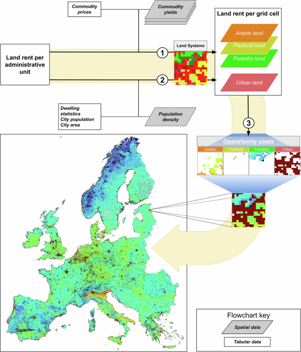
Opportunity costs of productive landAllocation procedure
For productive lands (i.e., agricultural land, including arable and pastural land, and forestry land), land rent data is available from the Nomenclature of Territorial Units for Statistics (NUTS) level 3 (sub-national administrative regions, like provinces) to level 0 (nations), depending on the country (for a breakdown of land rent data, see Table 1; for information on all input data sources, see Supplementary Table 2). We allocated the coarse-grain land rent data to the grid cell level of the land systems map (1 km) following the approach as described by Doelman et al. and Jantke et al.19,22. Essentially, we assume that in each grid cell the land rent value is proportional to the yield obtained, as (Eq. 1):
$${R}_{i,j}={R}_{j}\cdot \frac{{y}_{i,j}}{{\sum }_{i}^{n}({s}_{i,j}\cdot {y}_{i,j})}$$
(1)
where j denotes a (sub)national region with land rent data available, i denotes a grid cell within j, \({R}_{i,j}\) refers to the land rent allocated to a given grid cell in a given region (€/ha/yr), \({y}_{i,j}\) refers to the yield value of a grid cell within the region (€/ha/yr), \({R}_{j}\) denotes the regional land rent (€/ha/yr), and \({s}_{i,j}\) refers to the share of each grid cell in the total area of the same land type within region j (dimensionless). Since in our study all grid cells have the same area (1 km), \({s}_{i,j}\) is constant, hence we can equate \(\mathop{\sum }\limits_{i}^{n}{(s}_{i,j}\cdot {y}_{i,j})\) with the mean of the gridded yield values \({y}_{i,j}\) within a region j. The input data required for the opportunity cost estimation for productive lands include land rent data for arable land, pastoral land and forestry land (i.e., variable \({R}_{j}\) in Eq. 1) and spatially explicit monetary-based yield data for these land categories (i.e., variable \({y}_{i,j}\) in Eq. 1) (see Supplementary Table 2). We obtain the latter by multiplying yield data in biophysical units (kg/ha/yr) by the unit price of the commodity (€/kg/yr). In the following sections we further explain how we obtained and processed the land rent data and the yield data.
Table 1 Overview of the agricultural (i.e., arable and pastoral) land rent data sources and resolution.Land rent data
Arable and pastoral lands
Agricultural (i.e., arable and pastoral) land rent is defined as the price of renting one hectare of agricultural land during the reference period (a calendar year)23. Agricultural land rent represents the foregone income of agricultural land owners if the land is allocated for conservation and agricultural activities are abandoned13. For arable and pastoral lands, we obtained land rent data from the European Statistical Office (Eurostat)23 where available, and where not, we took values from the offices for national statistics24,25,26,27,28,29. Where we could not obtain agricultural land rent data from the offices for national statistics, we obtained agricultural land rent values from the Modular Applied General Equilibrium Tool (MAGNET)19. The resolution of the compiled agricultural land rent values varies from the NUTS 3 level to the supra-national level of the MAGNET regions (Table 1). In the Eurostat dataset, rent data are available for three categories: arable land, permanent grassland, and arable land/permanent grassland, where the latter are an average of the arable and permanent grassland rents23. Where available, we used land rent data specific to arable land or pastoral land (using the permanent grassland rents), and where not, we used the combined arable/permanent grassland rent values. The latter applied to 16 countries (AT, CZ, DK, EE, EL, ES, FI, FR, LU, LV, MT, NL, PL, SE, SI, and UK; for an overview of two letter country codes and corresponding countries, see Supplementary Table 3).
Statistics Portugal provides total agricultural land rent values at NUTS 2 level, instead of land rent values per unit area29. In the absence of NUTS 2 agricultural area values from Statistics Portugal, we converted these values to rent per hectare values based on the total area of cropland and grassland per NUTS 2 region, obtained from the land systems map. Similarly, the Federal Statistical Office of Switzerland provides the total agricultural land rent values per NUTS 3 region28, so we used the total agricultural area that was also provided by the Federal Statistical Office of Switzerland to determine the €/ha value for each NUTS 3 region30. For Wales and Northern Ireland, land rent data are available per hectare and per farm type, which does not necessarily conform to the arable-pastoral land split. Therefore, we used the average value across farm types as a combined agricultural land rent value. From the remaining countries with agricultural land rent data from national statistics offices (Scotland and Germany), only Germany had separate values for arable and permanent grassland land rents.
If land rent values were provided in a currency other than euro, we converted them to euros based on the exchange rate specific to the corresponding year. We then converted all land rents to 2021, which was the most recent year available in Eurostat23 at the time of analysis (i.e., first half of 2023), using a year-to-year Eurozone-specific annual inflation rate of the euro, referred hereafter as the nominal-to-real conversion31.
Forestry lands
In Europe, leasing forestry land is far less common than leasing agricultural land32, and so it is more appropriate to use the net economic benefits of forestry (profits or revenues minus production costs) as the proxy of opportunity cost of conservation in forestry land. We obtained forestry land rent data from the World Bank33, which provides rent data at the national level (i.e., NUTS 0) as a percentage of a country’s GDP for domestic timber and non-timber forestry production per year. We use the World Bank’s GDP data34 to convert the relative values to absolute monetary values for the year 2021 and then convert these values into a per hectare unit using the total area of wooded land per country according to Eurostat35. We took all values from 2021, and like the agricultural land rent data, we converted non-euro currencies to euros. The forestry rent dataset covers all European countries except six (i.e., Andorra (AD), Liechtenstein (LI), Kosovo (XK), Malta (MT), San Marino (SM) and the Vatican City (VA)). For countries without forestry rent values yet containing forest land according to the land systems map36, we used the average forestry land rent across all neighbouring countries with data available. We defined neighbours as countries sharing terrestrial or maritime borders, as follows: for Andorra, ES and FR; for Liechtenstein, AT and CH; for Malta, EL and IT; for San Marino, IT; for Kosovo, AL, RS and MK (see Supplementary Table 3 for country codes).
Yield data
Arable land
To obtain yield data for arable land, we combined gridded crop yield data (kg/ha/yr) with the country-specific unit price per crop (€/kg). We obtained crop yields from the Spatial Production Allocation Model 2010 (MapSPAM) (v2) dataset37,38, which provides spatially explicit yield data at a 5 arc-minute resolution (approximately 10 km at the equator) for 42 crop categories. We included all MapSPAM crop categories that are produced in Europe, according to The Food and Agriculture Organization Corporate Statistical Database (FAOSTAT)39 and MapSPAM37,38, and with crop price data available (Supplementary Table 5). We used the total crop yield per cell (kg/ha/yr) across all farming technologies included in MapSPAM (irrigated, rainfed high inputs, rainfed low inputs, rainfed subsistence and rainfed), obtained as harvested area weighted average of the four farming technology yields37. We resampled the MapSPAM layers to the projection and resolution of the land systems map (ETRS LAEA EPSG:3035, 1 km), using nearest neighbour and bilinear resampling, respectively.
We obtained crop producer prices for the years 2001 to 2021 from Eurostat40 and FAOSTAT41, available at the country (NUTS 0) level. Primarily, we used the crop producer prices from Eurostat (€/t)40, either for the year 2021 when available or for the first available preceding year. In absence of producer prices in Eurostat, we took country-level FAOSTAT producer prices41, which are provided in US dollars per tonne (USD/t). Crop price data were missing for three countries (CY, XK and ME). For these countries we used an average of the prices of neighbouring countries (i.e., for Kosovo from RS, AL and MK; for Montenegro from BA, RS, and AL; and for Cyprus from EL, since this is the only European country sharing a (maritime) border with CY). Similar to the land rent data, we first converted non-euro currencies to euros and then standardised all values to 2021 levels using year-to-year inflation rates31. Finally, we converted prices per tonne to prices per kg for consistency with the MapSPAM data.
To combine the yield and the price data, we matched the MapSPAM crop categories, which are based on the FAOSTAT system of crop categorisation, with the Eurostat system of crop categorisation (Supplementary Table 5)42. For MapSPAM crop categories that correspond to multiple crops in the crop price dataset, such as temperate fruit, we averaged the prices across the corresponding crops. Finally, we averaged the monetary yield values across the crop categories present in a grid cell to obtain a single monetary crop yield value per grid cell, as (Eq. 2):
$${y}_{a,i,j}=\frac{{\sum }_{1}^{c}{y}_{c,i,j}\cdot {p}_{c,j}}{{n}_{c,j}}$$
(2)
where \({y}_{a,i,j}\) is the monetary yield of arable land in grid cell i in region j (€/ha/yr), \({y}_{c,i,j}\) is the yield of crop category c in grid cell i in region j (kg/ha/yr), \({p}_{c,j}\,\) is the unit price of crop category c in country j (€/kg) and \({n}_{c,j}\) is the number of crop categories c present in country j according to MapSPAM and where price data is available according to the Eurostat40 and FAOSTAT41.
Pastoral land
We quantify the yield of pastoral land based on livestock production. Since livestock production data is only available at the country level (NUTS 0)43,44, we used the livestock density data from the Gridded Livestock of the World (GLW4) database (year 2015)45,46,47,48 to account for within-county variability. We assumed that pastoral land is occupied primarily by grazing animals and therefore selected grazing ruminant livestock from the GLW4 dataset: cattle, goats, and sheep. We excluded horses assuming their contribution to livestock products (meat and milk) is negligible. While reindeer are an important source of meat and milk in Nordic countries, we could not include them because they are absent from the GLW4 data. In addition, reindeer are typically allowed to roam freely, including in protected areas, hence setting aside land for nature conservation does not come with opportunity costs49. The GLW4 dataset has a spatial resolution of 5 arc-minutes (approximately 10 km at the equator) and includes dasymetric and areal-weighted livestock density maps (expressed in heads per 10 km) (see Supplementary Table 2 for all pastoral land inputs). We selected the dasymetric version because of its more realistic distribution patterns45. Since the GLW4 maps are in the same projection and resolution as the MapSPAM maps, we took the same approach to resample the maps to align the resolution and projection to the land systems map. We then divided the result by 1,000 to convert the units from heads per 10 km to heads per hectare, assuming homogenous distribution of livestock with the larger 10 km grid cell.
Next, we estimated the yearly monetary value per head of cattle, sheep and goats (€/head/yr). To that end, we quantified the total monetary yield per livestock species per region per year, and divided this by the total number of animals of that species per region, as (Eq. 3):
$${y}_{l,j}=\frac{{\sum }_{1}^{q}{y}_{q,l,j}\cdot {p}_{q,l,j}}{{\sum }_{1}^{i}{n}_{l,i,j}}$$
(3)
where \({y}_{l,j}\) is the monetary yield of livestock species l in region j (€/head/yr), \({y}_{p,l,j}\) is the yield of product q (milk or meat) obtained from livestock species l in region j (in kg/yr), \({p}_{q,l,j}\) is the unit price of product q (milk or meat) obtained from livestock species l in region j (in €/kg), and \({n}_{l,i,j}\) is the number of animals of livestock species l in cell i in region j (heads), as obtained from the GLW4 data.
We obtained the total annual production estimates of milk and meat per livestock species per country from Eurostat43,44, which were available for nearly all countries (except Kosovo). Where 2021 values of production were not available, we took the value from the most recent year reported. We obtained unit producer prices (€/kg) from Eurostat50 and FAOSTAT41 for the meat and milk of cattle, sheep, and goats. We note that the availability of price data was higher for cattle than for goats and sheep. We missed producer prices for all livestock species from Montenegro, Serbia, and North Macedonia, and since these countries neighbour each other, we took an average of the producer prices across the countries in the Central Europe MAGNET region. For Kosovo, we missed both production and price data, and we used the livestock-specific €/head value from Albania, which was the only neighbouring country with price and production data. San Marino and Andorra also missed price and production data, and therefore we used the Italian values and an average of the French and Spanish values, respectively.
Next, we multiplied the monetary yield per head values with the GLW4 gridded population maps to obtain gridded livestock monetary yield maps per livestock species (€/ha/yr), as (Eq. 4):
$${y}_{l,i,j}={y}_{l,j}\cdot {d}_{l,i,j}$$
(4)
where \({y}_{l,i,j}\) is the monetary yield of livestock species l in grid cell i in region j (€/ha/yr), \({y}_{l,j}\) is the per capita yield of livestock species l in region j (€/head/yr) as obtained with Eq. 3, \({d}_{l,i,j}\) is the population density of livestock species l in grid cell i in region j (heads/ha) as obtained from the GLW4 map. Finally, we averaged the yield data across the livestock species present in a grid cell to arrive at the total monetary pastoral yield per grid cell. We excluded a species if there was no data on commodity prices.
Forestry land
We obtained timber yield values in monetary terms by multiplying grid-specific woody biomass yield values (available in 1000m3/km/yr) by the export timber prices per country (available in €/1000m3), as (Eq. 5):
$${y}_{f,i,j}=\frac{{y}_{t,i,j}\cdot {p}_{t,j}}{100}$$
(5)
where \({y}_{f,i,j}\) is the monetary yield of forestry land in grid cell i in region j (€/ha/yr), \({y}_{t,i,j}\) is the monetary timber yield in grid cell i in region j (1000m3/km/yr), \({p}_{t,j}\) is the unit price of timber-based product (roundwood, sawnwood, wood pulp or a weighted mean of sawnwood and wood pulp based on national production outputs) in country j (€/1000m3), and the division by 100 is to convert from km to ha.
We retrieved gridded woody biomass yield data from the wood production dataset by Verkerk et al.51,52. They downscaled national wood production statistics (years 2000–2010) for 29 European countries to a 1 km resolution using a regression model that estimates forest yield based on various location characteristics, including climate (precipitation, temperature), terrain ruggedness, productivity and tree species composition. We used the latest map available in the dataset, i.e., the annual wood production of 2010, which is in the ETRS89-extended LAEA projection. The projection and resolution of this map are already aligned to our land systems map. The wood production map omits Malta and the Western Balkan states (HR, RS, ME, MK, BA, AL, XK). For the omitted Western Balkan countries, we used average wood production values based on the other nations that are in the MAGNET Central Europe region, and for Malta we took the value from IT.
We obtained roundwood, sawnwood and wood pulp export timber prices (2020USD/1000m3) from UNECE/FAO53, and converted these into 2021 euro values based on the 2020USD to 2020EUR exchange rate and the inflation rate of the euro from 2020 to 2021. Preferably we used both sawnwood and wood pulp price data, and combined these values using the ratio of the respective wood product type (“Sawlogs and veneer logs” and “Pulpwood, round and split”) removals reported by Eurostat54 as the weights. However, if either price were not available, we used roundwood prices as a substitute, as both sawnwood and wood pulp come under the umbrella of roundwood according to the FAOSTAT Forest Product Production Statistics55. If roundwood export prices were not available, but either one of sawnwood or wood pulp prices were available, we used the available one as the wood product price. Finally, if no prices were available, we substituted the export prices based on averages across neighbouring countries. Wood price data were missing for six countries (AD, CY, LI, XK, MT and MK). We used the following neighbouring country(s) average: for Andorra, FR and ES; for Cyprus, EL; for Liechtenstein, AT and CH; for North Macedonia, AL, BG, RS, EL; for Malta, IT; for SM, IT; for Kosovo, RS, AL and ME. We preferred to use wood product prices that are representative of the type of wood products that drive production in a region and prices that reflect the earliest stages of the manufacturing process of these products. Pulpwood prices (i.e., for the wood) would have been preferable over wood pulp prices (i.e., for the derived product), but the former were not available in consistent price forms for different countries. Therefore, we chose to use export prices for wood pulp.
Urban land rent
We approximated opportunity costs for urban land by the rent paid by a tenant to a property owner. We first obtained area-standardised residential rent values available for a sample of European residential areas (n = 42), and then established a linear regression model that relates these rent values with population density and major European region (North, East, South and West, following the regional divisions made by Dou et al.56) to extrapolate residential rents to all residential areas in the land systems map. The rent dataset includes monthly residential rent values for all capital cities across the European Union and Switzerland for 2021, six additional cities (CH: Genève; IT: Varese; DE: Bonn (2020), Karlsrühe and München) and one village (UK: Culham)57. The rent values are specified for different dwelling types: non-detached house, detached house and 1-, 2-, and 3-bedroom flats. As for all monetary-based datasets used in this study. We then converted the monthly values into yearly values to get the annual rent per urban area per dwelling type (€/yr). Converting these rents into per-hectare values requires information on the total number of each dwelling type per urban area. As this information was not available, we made an estimate based on the total population per urban area, the proportion of its population per dwelling type, and the typical household size, as (Eq. 6):
$${N}_{d,m}=\frac{{f}_{d,m}\cdot {P}_{m}}{{H}_{d}}$$
(6)
where \({N}_{d,m}\) is the number of units per dwelling type d in urban area m, Pc is the total population in urban area m, \({f}_{d,{m}}\) is the fraction of the population in dwelling type d in urban area m, and \({H}_{d}\) is the typical household size in dwelling type d.
We obtained the total population per urban area from Eurostat58, UN statistics59 and national and municipal statistics offices59,60,61,62,63,64,65,66,67,68. If available we preferred Eurostat data, thereafter data from UN statistics and again thereafter data from national and municipal statistics offices. Total population values were available for different years, ranging from 2011 to 2017; we took values for the latest year possible. For the proportion of the population in different dwelling types, we used country-level data from Eurostat (2018 to 2021)58. Since this dataset distinguishes only houses and flats, we aggregated the dwelling types into these two groups, and averaged the rents. As data on household size was not available, we assumed typical household sizes for houses and flats to be four (a family with two kids) and two (a couple), respectively.
Next, we multiplied the estimated number of units per dwelling type per urban area by the corresponding yearly rent per dwelling type, summed this across dwelling types, and divided by the total size of the urban area to find the total yearly rent per urban area on a per-hectare basis (Eq. 7):
$${R}_{m}=\frac{{\sum }_{1}^{d}{r}_{d,m}\cdot {N}_{d,m}}{{A}_{m}}$$
(7)
where \({R}_{m}\) is the area-standardized yearly residential rent in urban area m (€/ha/yr), \({r}_{d,m}\) is the average yearly rent for dwelling type d in urban area m (€/yr), \({N}_{d,m}\) is the total number of dwellings of type d in urban area m (Eq. 6), and Am is the size (ha) of urban area m. We obtained values on size from Eurostat and national and municipal statistical offices65,66,67,69,70,71,72,73,74.
We then fit a regression model relating the area-standardised yearly rents to the population densities of the residential areas per major European region (north, east, south and west), the latter to account for systematic differences in rent among regions. We obtained the population densities by dividing the total population size of each urban area (Pm in Eq. 6) by its area size (Am in Eq. 7). We log-transformed the area size and population densities because of their skewed distribution and we tested multiple model variants, selecting the most appropriate model based on the residual plot and on Akaike’s Information Criterion (AIC; see Supplementary Table 6 and Supplementary Figure 1). Finally, we used the regression model to estimate rent values for all residential areas in the land systems map, using as input population density estimates for 2020 that spatially comply with the land systems map75.
Integrating and standardising opportunity cost layers across land types
Finally, we combined the opportunity cost layers for the four land systems into a single layer. We assumed that the opportunity costs of conserving economically unproductive natural lands (land systems map classes are: bare, rock and shrubs; wetlands; water and glacier) are negligible and set these to zero. To assign opportunity costs to mosaic classes (Forest/shrub and cropland mosaic; Forest/shrub and grassland mosaic), which account for roughly 20% of the land systems map, we determined the share of every named land class in each mosaic cell using the high-resolution input of the land systems map, the Corine Land Cover (CLC) map (2018)36,76. We first resampled the CLC map from its original 100 m resolution to a 1 km resolution and then determined the percentage cover of each land category within a given mosaic class cell (see Supplementary Table 1 for land categories). We then quantified the opportunity costs of the mosaic classes proportional to the cover of the constituent classes.
The resulting combined layer reveals clear differences in opportunity costs between land types as well as between different regions in Europe (Fig. 2). As this regional variation may bias the results of spatial conservation prioritisation to regions with lower opportunity costs, we also provide two standardised layers. First, we standardised the average opportunity cost values within each country via standard-score (Z-score) normalisation. Second, we standardised the layer based on Eurostat purchasing power parities (PPPs) of national GDPs of each country for 202177. We standardised across countries using the same method as Pirson et al.78, where we obtain EU-PPP standardised values by dividing the euro estimates by the corresponding PPP values of each country.
Fig. 2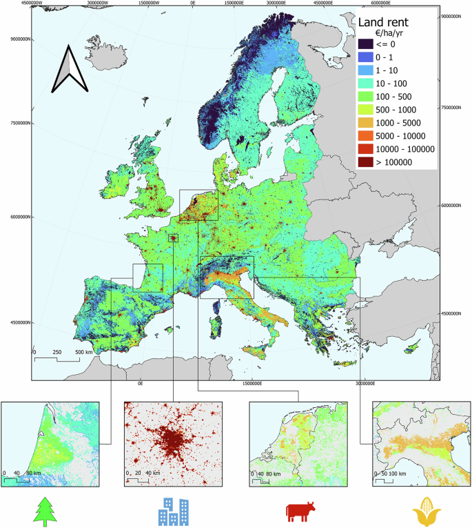
Opportunity costs of conservation across terrestrial Europe. Insets show examples of opportunity costs specific to forestry, urban, pastoral, and arable land (bottom left to bottom right).