
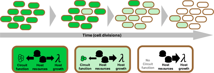
Modelling and quantifying gene circuit evolution
We develop an ordinary differential equation model of host-circuit interactions31,33 and augment it with a model describing an evolving population of E.coli cells, taking a similar state-transition approach to ref. 34 and ref. 30. This multi-scale model comprises a set of competing populations sharing a single source of nutrients, with each population representing a different parameterisation (or “strain”) of an engineered E. coli cell. Mutation is implemented via transitions between these different strains, and selection emerges dynamically through differences in calculated growth rates. Simulations are performed in repeated batch conditions, where nutrients are replenished and population size is reset every 24 hours, mirroring previous experiments4,10. Variables are given in molecules per cell (mc/cell). The complete model is defined in Supplementary Note 1. We perform simulations as defined in the Methods section entitled “Simulating an evolving population of engineered cells”.
Here, we consider a simple synthetic process consisting of a single gene A, which could represent a fluorescent reporter protein such as GFP. Messenger RNA (mRNA) transcripts mA are generated proportional to the maximal transcription rate ωA. They combine with ribosomes R supplied by the host model to form “translation complexes” cA, which yield protein pA upon the completion of translation, having consumed cellular anabolites e. Through consumption of e and utilisation of R the host and circuit models become coupled and the phenomenon of burden is captured32. We define the total output of the system P to be the total number of molecules of pA across the entire population composed of i strains:
$$P={\sum}_{i}\left({N}_{i}{{p}_{A}}_{i}\right),$$
(1)
where each strain i represents a different mutant, and Ni is the number of cells belonging to the ith strain (Fig. 2a). For this nominal open-loop system, we assume four distinct “mutation states” which differ in the value of the maximal transcription rate ωA, corresponding to 100%, 67%, 33% and 0% of the nominal or designed level. Mutation occurs via transition rates between these populations such that only function-reducing mutations may occur, and such that more extreme mutations are less likely (Fig. 2b). (See Supplementary Note 1 and Supplementary Fig. S1 for a full description of the mutation scheme.)
Fig. 2: Simulating an open-loop process in repeated batch conditions.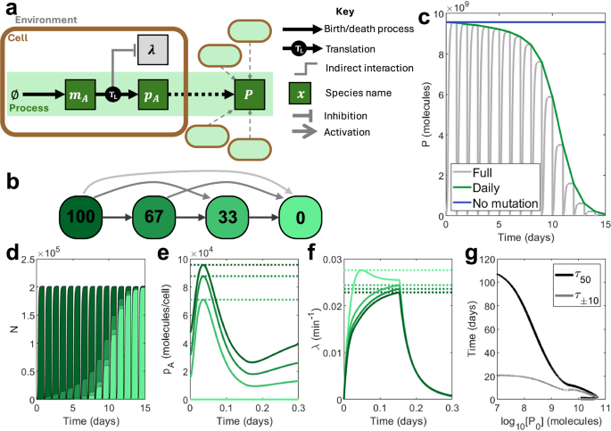
a A schematic showing the function of the process. mA is spawned and translated to create output pA using host ribosomes. This process impacts host growth. The total output P comes from the output pA across an entire population of engineered cells. b A visual depiction of the mutation scheme for this process. Coloured squares represent distinct ‘mutation states’ with different levels of function. Numbers in the squares show the percentage function of a given state relative to the designed level, implemented through differences in the maximal transcription rate ωA: 100 represents a state functioning as designed, while 0 represents a completely non-functional state where no transcripts mA are produced. Arrows signify possible transitions between mutation states, with lighter arrows representing mutations which occur less often. c‒f Time-series outputs using an open-loop process with maximal transcription rate \({\omega }_{A}=5\,\,{\mbox{mc}}\,\,{\min }^{-1}\). c Total population-wide circuit output P, plotted both in full (grey) and at the end of each simulation day (green). An ideal system would match an open-loop system in the absence of mutation, maintaining function indefinitely (blue). d Population size N, distributed according to mutation state. Dark green represents a fully-functional (100%) strain. Light green represents a non-functional (0%) strain. e Output per cell pA according to mutation state over the first day. Dotted lines show maximum outputs. f Growth rate λ according to mutation state over the first day. Dotted lines show maximum growth rates. g For a wide range of processes (varying ωA between 0.1 and 1000 mc min−1), τ±10 (black) and τ50 (grey) against initial output P0. Simulation results are provided as a Source Data file.
To measure the evolutionary longevity of this process, we define three metrics:
1.
P0, the initial output P from the ancestral population prior to any mutation.
2.
τ±10, the time taken for the output P to fall outside of the range P0 ± 10%.
3.
τ50, the time taken for the output P to fall below P0/2.
We define these metrics assuming that we wish to maximise production (P0) and maintain performance near to the original state (τ±10) for as long as possible. We propose τ50 as a measure of long-term performance or “persistence” because the maintenance of “some function” may be sufficient for many applications, such as biosensing.
For the proposed nominal open-loop system, the total output P falls over the course of the simulation from its initial value P0 to 0 molecules (Fig. 2c). This corresponds to a transition of the population makeup, which initially comprises entirely of fully functional cells but eventually is dominated by non-producing, faster growing mutants (Fig. 2d–f). For systems with increased process transcription (i.e., larger maximal transcription rates ωA), the initial output P0 increases as more protein is produced per cell. However, this increases the burden caused by the process and therefore reduces both τ50 and τ±10. Beyond a certain point, continuing to increase ωA can overburden the cell, leading to a reduction in all metrics (Fig. 2g).
The objective of this paper is to evaluate the ability of different control strategies to improve the evolutionary longevity of this simple synthetic circuit. It is trivial to reduce the burden and improve both τ±10 and τ50 by reducing the production of pA via the birth rate ωA. However, this impedes circuit function (Supplementary Fig. S2a). We therefore define the performance of controllers in comparison to an open-loop system of equal initial output P0. See Methods for Comparing controllers versus open-loop systems of equal output for full details as to how these metrics where determined. The ideal controller would extend τ±10 and τ50 at no loss in P0.
Phenomenological models demonstrate the potential of negative feedback control to enhance evolutionary longevity
We consider three candidates for the choice of input for a control strategy designed to improve evolutionary longevity (Fig. 3a). We model all controllers phenomenologically by scaling the maximal transcription rate of the circuit gene ωA by a regulatory function, so that protein production is inhibited when levels are already high:
$${w}_{A}={\omega }_{A}\cdot \Theta (u).$$
(2)
Here, u is the control input of choice.
Fig. 3: Phenomenological modelling of different choices of control input.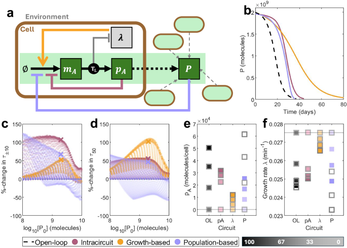
a A simple schematic showing the three controller architectures: intra-circuit control (red), growth-based control (orange) and population-based control (lilac). Each output comes from a different layer of the combined multi-scale model (circuit model, host model and population model). See key in Fig. 2a for symbol meanings. b Time-series of population-wide output P over time for an open-loop system (black, dashed, wA = 4.0 mc min−1) and representative control systems of equivalent initial output P0. (Intra-circuit: red, wA = 103 mc min−1, kA = 4.5 × 10² mc. Growth-based: orange, wA = 87 mc min−1, kλ = 6.3 × 10⁻² min−1. Population-based: lilac, wA = 16 mc min−1, kP = 5.2 × 10⁸ mc.). c, d A large number of designs were generated by varying the maximal transcription rate ωA and control parameters ku. Against the initial output P0, we plot the percentage change in (c) τ±10 and (d) τ50 vs an open-loop system of equal initial output. Points marked with an X correspond to the time-series plots in (b). These were selected as points on the Pareto fronts simultaneously optimising P0, τ50 and τ±10, with initial output P0 closest to 2 × 10⁹ molecules. e, f For circuits corresponding to trajectories in (b), (e) maximum protein production per cell pA and (f) maximum growth rates λ across the first day (solid) and the day where τ50 is reached (grey outline) for each mutation state. Lighter squares represent less functional strains. The horizontal line represents a non-functional strain. Simulation results are provided as a Source Data file.
Firstly, we consider product-based negative feedback where the protein per cell pA is the control input (Fig. 3a, red). To maintain function close to a desired level, production is inhibited if there is an abundance of output and control is alleviated if production is low. We call this intra-circuit feedback. This is achieved via the regulatory function:
$$\Theta ({p}_{A})=\frac{{{k}_{A}}^{2}}{{{k}_{A}}^{2}+{p}_{A}^{2}}.$$
(3)
Should a mutation occur which reduces the production of pA, the strength of control will be eased, allowing the actual output levels to rise again. This means that mutations which reduce circuit output will have a lesser impact on burden, minimising the selective advantage of such mutations.
Secondly, we consider growth rate λ as the control input (Fig. 3a, orange). Since increased production of pA corresponds to reduced growth, we employ feedback so that production is inhibited at low growth. We call this growth-based feedback, and use the regulatory function:
$$\Phi (\uplambda )=\frac{{\uplambda }^{2}}{{{k}_{\uplambda }}^{2}+{\uplambda }^{2}}.$$
(4)
If a burden-relieving mutation arises with reduced production of output pA, control will be alleviated, enabling a resultant increase in output and a smaller selective advantage over the original designed strain.
Finally, since our objective is to maintain the performance of a synthetic circuit across an entire population, we consider using the total population-wide output P as an input for control (Fig. 3a, lilac). Such a system could be implemented physically using cell-to-cell communication systems such as quorum sensing. We employ feedback so that further production is inhibited when the population-wide output P is high. We call this population-based feedback, and use the regulatory function:
$$\Theta (P)=\frac{{{k}_{P}}^{2}}{{{k}_{P}}^{2}+{P}^{2}}.$$
(5)
Unlike with the other systems, individual cells do not directly respond to mutations in the circuits they carry by alleviating control, because such mutations do not significantly alter the population-level control input P. Instead, this system aims to maintain population-level output by steadily increasing the per-cell production of non-mutant cells to compensate for the increasing number of non-functional mutants.
For all three systems, applying control to a given nominal process (here, ωA = 10 mc min−1) boosts longevity at the expense of initial output P0, with stronger controllers (low kA, high kλ, low kP) causing a more significant change (Supplementary Fig. S2b‒d). Representative dynamics from systems which initially produce the same population-wide output P are shown in Fig. 3b. This initial comparison suggests that intra-circuit control is capable of maintaining function at close to the designed level for longer (greater τ±10), but that growth-based control is more effective at improving long-term persistence (greater τ50). To assess the different strategies at the topological level, we generated many designs by varying both the process input ωA and the controller strength (kA, kλ and kP) while all other system parameters were fixed as defined in Supplementary Table 4. We observe that intra-circuit control excels in the short term while growth-based control excels in the long term across most parameter combinations, demonstrating that the result holds at the topological level (Fig. 3c, d). Except in cases of minimal output, population-based control is less effective and is the only strategy where some designs perform worse than open-loop. These differences in performance are a result of differences in the per-cell protein production and growth rates between mutant strains (Fig. 3e, f). For intra-circuit control, mutating into intermediate mutation states (where function is non-zero but less than the designed level) alleviates some of the control exerted by the controller, pushing production back up and providing a smaller growth advantage. However, this means that mutations which completely abolish function provide a greater growth advantage, allowing non-functional mutants to dominate quickly, accelerating loss-of-function. Growth-based control is capable of boosting the growth rate of the fully-functional state, thereby reducing the selective advantage of mutation into any other state. For population-based control, non-mutant cells become affected by a decline in population-wide output, so that control strength is eased over time. This allows them to produce more output, but leads to an even greater selective disadvantage, thereby accelerating loss-of-function.
Having established the theoretical differences in performance for different controller input strategies, we next consider how such systems could be implemented in living cells by deriving mechanistic models of biologically realisable topologies. We consider both transcription factor-based and RNA-based methods of control information processing and actuation. In the main text, we report the results for the intra-circuit and growth-based systems. Mechanistic modelling of a population-based controller which utilises quorum sensing confirms that such systems have poor performance (Supplementary Figs. S3‒S6). These results are described in Supplementary Note 2.
Intra-circuit feedback control improves short-term performance at the expense of longevity
The intra-circuit control strategy described in the above section and demonstrates the potential of negative feedback control to enhance evolutionary longevity (Fig. 3) is equivalent to an autoregulation motif where an inhibitory transcription factor inhibits itself. This limits its utility in practice, where one may want to stabilise the expression of an enzyme or signalling protein that performs a useful circuit-specific function. Here, we consider two biologically implementable control systems where feedback is enacted in proportion to the per-cell protein output pA. The first is composed of an inhibitory transcription factor pB, which is produced from the same promoter as circuit protein pA, so that the functional identity of pA is not constrained. pB inhibits the production of both pA and pB (Fig. 4a). In this way, when production is high, increased inhibition reduces the production of new synthetic proteins, enabling the reduction of burden. This approach imitates previously implemented controllers (such as ref. 26). We call this controller CLpATX (“Closed-loop, senses pA, prevents transcription”). To implement this, we scale the birth rate of mRNAs by the regulatory function:
$${\Theta }_{A}(\,{p}_{B})=\frac{{{k}_{B}}^{2}}{{{k}_{B}}^{2}+{{p}_{B}}^{2}}.$$
Note that the controller protein here will exert an additional burden on top of the process gene.
Fig. 4: Protein-based control design and performance.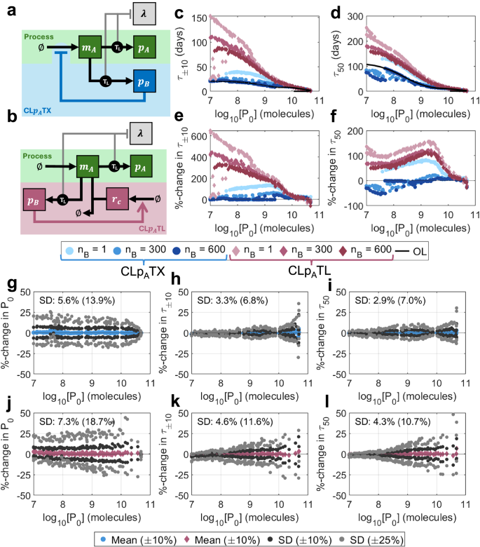
a A schematic describing the controller CLpATX. Controller protein pB is produced from the same gene as output protein pA and acts as an inhibitory transcription factor on the shared gene. b A schematic describing the controller CLpATL. See key in Fig. 2a for symbol meanings. A controller protein, pB, is produced from the same gene as the output protein pA, and acts as a transcription factor which activates the production of sRNA rC. The feedback loop is completed through the combining of rC with mRNA that codes for pA and pB, preventing it from being translated. c‒f Optimal performance for both CLpATX (blue) and CLpATL (red) for controller protein length nB = 1, 300, 600 aa. c τ±10 vs initial output P0, (d) τ50 vs initial output P0, (e) %-change in τ±10 over open-loop vs initial output P0, (f) %-change in τ50 over open-loop vs initial output P0. g‒l Robustness analyses for (g‒i) CLpATX and (j‒l) CLpATL. For each of the 100 optimal controllers with nB = 300 aa, 100 further controllers were generated by varying parameters by up to ± 10% (dark grey) and ± 25% (light grey). The percentage changes in three output metrics were calculated versus the original optimal systems: (g, j) P0, (h, k) τ±10 and (i, l) τ50. Plots show the means (for ± 10%) and standard deviations (for both ± 10% and ± 25%) of the percentage changes for each optimal controller. Percentages marked on the plots indicate the standard deviations across the entire Pareto front when parameters were varied by ± 10%(± 25%). Simulation results are provided as a Source Data file.
The second negative feedback mechanism similarly makes use of a co-produced transcription factor pB, but in this case it activates an sRNA rC which then eliminates the mRNA mA by sequestration (as in e.g.35) (Fig. 4b). We call this controller CLpATL (“Closed-loop, senses pA, prevents translation”). (For ease of reference, the names of the controllers, their inputs and mode of action are available in Supplementary Table S1). Note that there are now two genes which may be subject to mutation (the process and the sRNA) and so we update our mutation model to include 42 = 16 distinct mutation states, where each represents a unique pair [%A, %C], with %A, %C ∈ {100%, 67%, 33%, 0%}. We assume that mutations only affect a single promoter at a time (Supplementary Fig. S1). (See Supplementary Note 1 for a full description of both models for a full description of the mutation scheme.)
We first consider the transcriptional controller architecture: CLpATX. To determine its performance across a range of processes, we performed multi-objective optimisations to simultaneously maximise P0, τ±10 and τ50, varying the control strength kB, the control protein ribosome binding rate bB and the circuit maximal transcription rate ωA (see Methods section “Multi-objective optimisation”). To evaluate performance, we then compared these outputs with corresponding open-loop systems of equal initial output P0. (See Methods section “Comparing controllers versus open-loop systems of equal output”).
For controller protein lengths typical of bacterial regulators (i.e., nB = 300 amino acids (aa)), improvements in τ50 are minimal, but τ±10 can be improved by up to 60% versus open-loop (Fig. 4c–f, blue). Our optimisations show that, where improvements are possible, control strength should be maximised (i.e., low kB) across the Pareto front (Supplementary Fig. S7, blue). This is because stronger inhibitors do not need to be as abundant to achieve the same strength of feedback, and so controller burden can be minimised. At low outputs P0, where performance increases are minimal or non-existent, controller binding strength bB is very small, so there is less pressure to minimise kB as controller proteins are less abundant. Systems which produce less output (and have increased longevity) tend to have less synthetic transcription (low ωA) and less controller translation (low bB) (Supplementary Fig. S7, blue).
We tested the robustness of the optimal designs to parametric uncertainty by varying the optimal parameters randomly by up to ± 10% to generate 10,000 alternate designs. We repeated the analysis for ± 25%. To quantify robustness, we tracked the percentage change in each metric (P0, τ±10 and τ50) versus its corresponding optimal system. A robust architecture would have small standard deviations in these values when the designs across the Pareto front are subjected to variation (See Methods section “Robustness analysis”). Here, optimal controllers are very robust to parametric variation, with changes in P0, τ±10 and τ50 having standard deviations of 5.6% (13.9%), 3.3% (6.8%), and 2.9% (7.0%) respectively, compared with the original optimal systems when parameters were varied by ± 10% (± 25%) (Fig. 4g–i). (See Supplementary Note 3 for our comprehensive robustness analysis (Supplementary Fig. S8a‒d and Supplementary Table S2).)
In an ideal case where the repressor causes minimal burden (i.e., nB → 0 aa), performance can be significantly boosted to the levels suggested by the phenomenological models. The binding rate bB can be increased without significantly increasing burden (Supplementary Fig. S7, blue). However, increasing the repressor size nB to 600 aa, and therefore increasing controller burden, performance deteriorates to worse than open-loop and any benefits of control are lost entirely. As repressor size increases from 300 aa to 600 aa, the parametric design rules do not qualitatively change (Supplementary Fig. S7, blue).
To better understand how design choices impact this controller architecture, we tested the performance of this controller for a nominal process of maximal transcription rate ωA = 50 mc min−1 and controller protein length nB = 300 aa by varying the controller ribosome binding rate bB and the controller strength kB. We show that τ±10 can be improved by a more significant margin than τ50, and across a wider portion of the design space, suggesting that it is easier to boost short-term performance than long-term performance (Supplementary Fig. S9). (See Supplementary Note 4.)
Post-transcriptional control outperforms transcriptional control for intra-circuit feedback
Unlike CLpATX, which only enhances performance when controller size (and therefore burden) is minimal, CLpATL is capable of significantly improving both τ±10 and τ50, even in the presence of large controller sizes (nB = 600 aa) (Figs. 4c–h, 5a, red). For typical regulator lengths (nB = 300 aa), τ50 can be more than doubled, with τ±10 showing an even more extreme improvement at low initial outputs of up to + 400% versus open-loop. Although this system significantly outperforms CLpATX, the optimal control designs are less robust, with random parameter variation of up to ± 10% (± 25%) causing larger variations in output metrics: changes in P0, τ±10 and τ50 have standard deviations of 7.3% (18.7%), 4.5% (11.6%) and 4.3% (10.7%) respectively (Fig. 4j–l). (See Supplementary Note 3 for a comprehensive robustness analysis (Supplementary Fig. S8e–h and Supplementary Table S2).) As with CLpATX, maximising controller strength (i.e., minimising kB) is crucial to achieve the most control for the least burden for nB = 300 aa and nB = 600 aa. For nB = 1 aa, controller burden is much less significant, so pushing kB to its absolute minimum is less important. Producing sRNA rC does not result in an additional burden, and so maximising its production allows for the strongest control (Supplementary Fig. S7, red). The demonstrated improvements in longevity of CLpATL over CLpATX are a result of two key mechanisms: (i) reduced controller burden (at equivalent control strength) and (ii) the emergence of mutations to the controller itself (enabling the short-term growth of high-producing strains).
Fig. 5: Understanding the improved performance of CLpATL.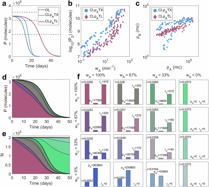
a–c Comparing CLpATX (blue) and CLpATL (red). a Population-wide process outputs P over time for two representative controllers. b Initial output P0 against the maximal transcription rate of the process gene ωA across all optimal controllers. c Controller protein per cell pB vs process output protein per cell pA across all optimal controllers. d–f The effect of controller mutation on CLpATL with nB = 300 aa. d Population-wide output P over time according to mutation state. e Population size according to mutation state. f Bar charts for CLpATL with nB = 300 aa showing (i) growth rate λ (min−1), (ii) process protein output per cell pA (molecules/cell) and (iii) sRNA per cell rC (molecules/cell). Each subplot represents a unique mutation state. Moving rightwards signifies mutation of the process, and moving downwards signifies mutation of the controller. Simulation results are provided as a Source Data file.
Firstly, we see that optimal controllers utilise larger maximal transcription rates ωA (Fig. 5b) and require much less controller protein pB than CLpATX (Fig. 5c). This is a result of the pB-mediated activation of rC, which amplifies the “impact” that each burdensome controller protein can achieve. This enables CLpATL to provide “more control for less burden” and significantly enhance performance in the long term.
Secondly, this process-controller system has two promoters (A driving the gene expression and C driving the controller). When the process promoter mutates (affecting the process transcription rate ωA), synthetic protein production falls, causing an increase in growth rate. However, when the sRNA promoter mutates (affecting the sRNA transcription rate ωC), the strength of control falls, so synthetic protein production rises, leading to a decrease in growth rate. Over time, the emergence of both types of mutation leads to a heterogeneous population of mutant strains, some of which produce more protein pA than the ancestral strain (Fig. 5d–f). It is important to note that there are two sources of mutant spread: (1) the emergence of new mutants via random mutation and (2) the competition between mutant strains as a result of their relative growth rates. In the long term, growth rate differences are the predominant cause of mutant domination; the higher-producing strains are outcompeted by faster-growing strains. However, early in the time course, when the majority of the population is still fully functional, the dynamics is primarily affected by the emergence of new mutations. Mutations to the controller can therefore initially balance out with mutations to the process, enabling function to be maintained close to the designed level for much longer, until out-competition becomes the dominant source of mutant spread. This effect also explains why the improvement in τ±10 is so high for smaller initial outputs P0: the differences in growth rate between mutants become much smaller, so the emergence of new mutants makes up a bigger proportion of the mutant spread, so cells with mutated controllers (and increased output) make up a larger fraction of the combined population, balancing out the cells with reduced process output. This results in a linear relationship between τ±10 and τ50 for optimal systems as the initial output P0 varies. This contrasts with CLpATX, where increases in τ±10 are more restricted than increases in τ50 at low outputs P0 (Supplementary Fig. S10a, e).
These higher-producing mutants are only prevalent in the short term but contribute significantly to the excellent short-term performance (τ±10) of CLpATL. The improvement in long-term performance over CLpATX is primarily a result of the reduced burden. To verify this claim, we separately considered a system with two dimensions of mutation but no additional burden. We observe improvements in short-term performance when we include a second controller-specific mutation site whose mutation leads to an increase in process output. However, long-term performance, optimal parameter choices and robustness are not significantly impacted (Supplementary Figs. S11 and S12). (See full details in Supplementary Note 5).
As with CLpATX, we explored how design choices influence performance for a nominal process (ωA = 50 mc min−1). As before, we see that τ±10 improves over a larger portion of the design space than τ50, demonstrating that short-term maintenance of function is easier to improve than long-term persistence (Supplementary Figs. S13 and S14). See Supplementary Note 4 for a full description.
We have shown that CLpATL outperforms CLpATX partly as a result of the low burden of transcription compared with translation. We extended our cell model to capture energy consumption, and therefore burden, by transcription. We found that CLpATX is insensitive to this additional burden and that CLpATL outperforms it except at the highest transcriptional burden (Supplementary Fig. S15). See Supplementary Note 6 for a comprehensive discussion. Given this observation, we proceed with the assumption that transcriptional burden remains negligible and that translational demands (in terms of both energy consumption and cellular resource competition) dominate bacterial growth and host-circuit interactions, in accordance with established models and experimental data19,31,36,37,38.
Growth-based feedback enhances evolutionary longevity
Synthetic circuit burden elicits the upregulation of specific natural promoters, which can be considered to be burden sensors. These promoters can be exploited to design control systems that are sensitive to burden39. When burden is high and growth is low, greater restriction on the process can alleviate burden and reduce the selective benefit of mutations to the process gene. As with intra-circuit control, we considered two growth-based controller designs: CLλTX (“Closed-loop, senses λ, prevents transcription”) (where control is exerted by an inhibitory transcription factor) and CLλTL (“Closed-loop, senses λ, prevents translation”) (which exploits sRNA-mediated mRNA sequestration). Both CLλTX and CLλTL improve evolutionary performance, with CLλTL outperforming CLλTX in both the short term (greater τ±10) and long term (greater τ50 except at very high initial outputs P0) (Supplementary Fig. S16). Here, we focus our analysis on CLλTL, with the discussion of CLλTX presented in Supplementary Note 7 (Supplementary Figs. S16 and S17). This controller exploits growth-sensitive promoters to drive transcription of an sRNA rC (Fig. 6a). When the cell undergoes stress (i.e., low growth rate), a controller protein pB is produced, which activates sRNA expression (rC). This sRNA combines with and eliminates the mRNA for the process gene mA, preventing it from being translated. There are three promoters in this system, so we employ a mutation scheme consisting of 43 = 64 distinct strains corresponding to unique triplets {%A, %B, %C} with {%A, %B,%C} ∈ {100, 67, 33, 0} (Supplementary Fig. S1). (See Supplementary Note 1 and Supplementary Fig. S1 for a full description of the mutation scheme.)
Fig. 6: Optimal outputs for CLλTL.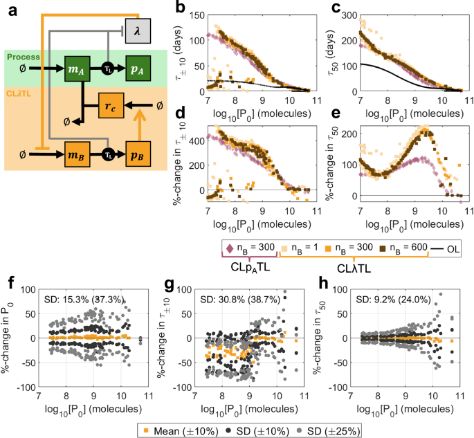
a A schematic describing the controller. Controller protein pB is produced from a growth-sensitive promoter and activates the production of sRNA rC. rC combines with and deactivates process mRNA mA. See key in Fig. 2a for symbol meanings. b–e Optimal performance for both CLλTL (orange) and CLpATL (red) for controller protein length nB = 1, 300, 600 aa. b τ±10 vs initial output P0, (c) τ50 vs initial output P0, (d) %-change in τ±10 over open-loop vs initial output P0, (e) %-change in τ50 over open-loop vs initial output P0. f–h Robustness analysis. For each of the 100 optimal controllers with nB = 300 aa, 100 further controllers were generated by varying parameters by up to ± 10% (dark grey) and ± 25% (light grey). The percentage changes in three output metrics were calculated versus the original optimal systems: (f) P0, (g) τ±10 and (h) τ50. Plots show the means (for ± 10%) and standard deviations (for both ± 10% and ± 25%) of the percentage changes for each optimal controller. Percentages marked on the plots indicate the standard deviations across the entire Pareto front when parameters were varied by ± 10%(± 25%). Only original optimal controllers where τ±10 = τ90 are considered. Simulation results are provided as a Source Data file.
For typical regulator protein sizes (nB = 300 aa), CLλTL slightly outperforms CLpATL in the short term, but significantly outperforms it in the long term, with possible improvements of more than 200% versus open-loop (Figs. 6b–e, 7a). The difference in performance in systems with minimal burden (nB = 1 aa) and high burden (nB = 600 aa) is very small, suggesting that this controller topology is less sensitive to controller burden than intra-circuit controllers. Observing the population dynamics, we see that when mutations affect the process gene, there is less variation in protein production and a minimal loss in growth rate, so mutant strains with reduced function have less of a selective advantage (Fig. 7b, d). Similarly, when mutations affect the controller, the new mutant strains with increased function have less of a selective disadvantage (Fig. 7c, e).
Fig. 7: Why does CLλTL outperform CLpATL?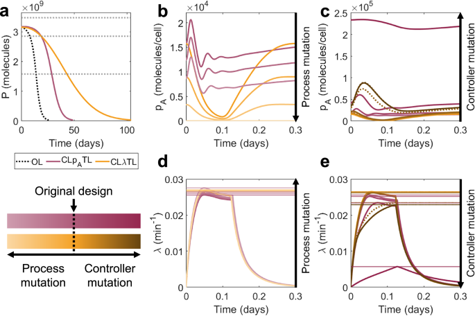
a Time-series output for representative optimal controllers with nB = 300 aa. (Open-loop black dotted line). b Protein output per cell pA over time for the first day of simulation according to mutation state, considering only states with a mutated process and a fully functional controller. c Protein output per cell pA over time for the first day of simulation, considering only states with a mutated controller and fully functional process (solid line mutation in ωB, dotted line mutation in ωC). d, e Growth rates λ according to mutation state. Main plots show time series over the first day. Horizontal lines indicate differences in the maximum growth rates of each state over the first day. d Only states with mutated process. e Only states with mutated controllers (solid line/square is mutation in ωB, dotted line/triangle is mutation in ωC). Simulation results are provided as a Source Data file.
Investigating the optimal controller designs shows only ωA has significant variation across the Pareto front. All other parameters demonstrate clear optimal choices across the performance space (Supplementary Fig. S17, orange). The strength of control from the transcription factor should be maximised (kB minimised). This becomes more crucial as protein length increases, corresponding also to a reduction in ribosome utilisation (reduced bB) but increased transcription of controller genes (increased ωB and ωC). kλ controls the sensitivity of the controller to changes in growth rate. Our optimisations show that controllers should have kλ in the region of 0.002 to 0.005 min−1, suggesting a high sensitivity to growth rate.
We note that some optimal systems with low initial outputs have τ±10 worse than open-loop. Investigating the system dynamics shows that these “fail” because their output increases significantly in the early stages of the simulation as a result of controller mutation (Supplementary Fig. S18a–c). These are systems for which the 90%-life τ90 (defined as the time taken for output to fall below 90% of its original value) is not equal to τ±10. These systems have low output and very strong controllers, so when the controller mutates, they produce a comparatively very large amount of output protein. Despite these strains with mutant controllers having very low growth rates and only arising in small numbers, their contribution to the population-wide output is significant (Supplementary Fig. S18e). The effect is enhanced by the existence of two separate controller genes, both of which can be mutated to yield this increase in output. This effect can be exploited to generate systems with excellent τ50 but poor τ±10 because of an initial increase in output before an eventual fall. This effect is more pronounced in systems with very low initial outputs P0, because the functional systems are less burdensome and therefore have less of a growth disadvantage (Supplementary Fig. S18f, g). This means that a greater proportion of mutant spread initially comes from the emergence of new mutants rather than competition between strains.
This phenomenon also makes this topology much less robust to parametric variation. In some cases, small variations in parameters can significantly and discretely alter the value of τ±10 as systems which previously remained below + 10% of the original value may now exceed it. Considering only the original designs where τ±10 = τ90, 21.6% (28.2%) of designs fail to maintain τ±10 = τ90 after parameters are randomly varied by up to ± 10% (± 25%). Standard deviations in the percentage change of P0, τ±10 and τ50 are 15.3% (37.3%), 30.8% (38.7%) and 9.2% (24.0%), demonstrating that, despite the improvements in long-term performance, this controller topology is much less robust than intra-circuit topologies (Fig. 6f–h). As with the intra-circuit systems, the post-transcriptional feedback mechanism (CLλTL) enables much greater optimal performance than the transcriptional feedback mechanism (CLλTX), but this comes at the expense of a reduction in robustness: for CLλTX, standard deviations in the percentage change of P0, τ±10 and τ50 are 9.1% (22.6%), 22.7% (35.9%) and 9.2% (17.4%) (Supplementary Fig. S16h–j). (See Supplementary Note 3 for a detailed robustness analysis of both controllers (Supplementary Fig. S19).) For systems where τ±10 = τ90, τ±10 and τ50 maintain a linear relationship (Fig. S10b, e).
To understand how design choices influence the performance of growth-based feedback systems, we considered how varying the controller parameters would influence the performance of CLλTX for a nominal process of ωA = 50 mc min−1. This is described in Supplementary Note 4. Unlike intra-circuit feedback, where it is easier to improve τ±10, growth-based feedback improves τ50 across a wider portion of the design space, suggesting that growth-based controllers could have greater potential for in vivo implementation in applications where circuit persistence is more important for maintenance of function close to the designed level (Supplementary Fig. S20).
We extended our analysis of growth-based control by considering a protein-free implementation where the growth-sensitive promoters drive the sRNA expression directly (rather than via a regulator protein). This system can improve performance versus open-loop but does not outperform CLλTL (Supplementary Figs. S21 and S22). See Supplementary Note 8.
Combining control schemes enhances robustness of growth-based feedback
We have shown intra-circuit control excels at maintaining short-term performance because it reduces the selective advantage of intermediate mutation states, whereas growth-based control excels at enhancing long-term performance because it boosts the growth rate of the fully functional state. Further, we have shown that sRNA-mediated controllers have enhanced optimal performance but poorer robustness than controllers which actuate directly via transcription factors. We therefore considered whether combining multiple inputs and mechanisms of feedback could combine the benefits of the individual systems and enable greater improvements in both longevity and robustness. We first considered a phenomenological model of a control strategy which utilises both product-based and growth-based control in conjunction. This system is described in Supplementary Note 9 and is capable of combining the benefits of both intra-circuit feedback and growth-based feedback to significantly enhance both short-term and long-term performance by up to 50% compared with the best performing single-input systems (Supplementary Fig. S23).
To assess the impact of biochemical constraints and controller burden on this strategy, we developed five multi-input mechanistic models which exploit both transcriptional and translational mechanisms of introducing feedback control: (i) CLpATLλTL uses protein-based feedback to inhibit transcription of the process gene and growth-based feedback to prevent translation of the process gene by activating sRNA (Fig. 8a), (ii) CLpATLλTX uses protein-based feedback to prevent translation of the process gene by activating sRNA and growth-based feedback to inhibit transcription of the process gene (Fig. 8b), (iii) CLpATLλTL uses both protein-based feedback and growth-based feedback to co-operatively activate sRNA production and prevent translation of the process gene (Fig. 8c), (iv) CLpATXλTX uses both protein-based feedback and growth-based feedback to co-operatively inhibit transcription of the process gene (Supplementary Fig. S24a) and (v) CLpATLλPF (PF := protein-free) uses both protein-based feedback and growth-based feedback to co-operatively prevent translation of the process gene by putting the sRNA gene directly on a growth-sensitive promoter (Supplementary Fig. S24b). Models for all five multi-input controllers are detailed in Supplementary Note 1.
Fig. 8: Designing multi-input controllers.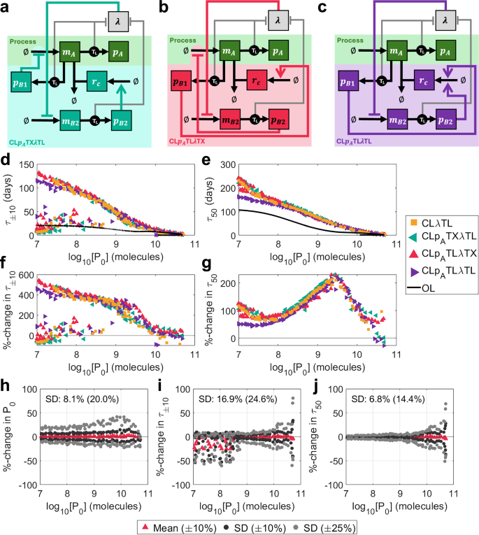
a–c Schematics of mechanistic multi-input controllers: (a) CLpATXλTL (protein-based inhibition of transcription, growth-based inhibition of translation, teal), (b) CLpATLλTX (protein-based inhibition of translation, growth-based inhibition of transcription, crimson), (c) CLpATLλTL (protein-based inhibition of translation, growth-based inhibition of translation, purple). See key in Fig. 2a for symbol meanings. d–i Optimised outputs for three multi-input controllers compared with CLλTL. (d) τ±10 vs initial output P0, (e) τ50 vs initial output P0, (f) %-change in τ±10 over open-loop vs initial output P0, (g) %-change in τ50 over open-loop vs initial output P0. h–j Robustness analysis for CLpATLλTX. For each of the 100 optimal controllers with nB = 300 aa, 100 further controllers were generated by varying parameters by up to ± 10% (dark grey) and ± 25% (light grey). The percentage changes in three output metrics were calculated versus the original optimal systems: (h) P0, (i) τ±10 and (j) τ50. Plots show the means (for ± 10%) and standard deviations (for both ± 10% and ± 25%) of the percentage changes for each optimal controller. Percentages marked on the plots indicate the standard deviations across the entire Pareto front when parameters were varied by ± 10%(± 25%). Only original optimal controllers where τ±10 = τ90 are considered. Simulation results are provided as a Source Data file.
Here, we present a discussion of systems (i–iii). We solved a multi-objective optimisation problem to identify Pareto optimal designs and found that the potential improvements gained from combining the control inputs are counteracted by additional controller burden, leading to only marginal improvements in performance versus CLλTL (Fig. 8d–g). The three multi-input controllers perform very similarly and obey similar primary qualitative design principles: maximise the production of sRNA (large wC), minimise the ribosome binding rate of the growth-sensitive protein \({{p}_{B}}_{2}\) (small \({{b}_{B}}_{2}\)), and maximise the strength of transcriptional control (small \({{k}_{B}}_{1}\) and \({{k}_{B}}_{2}\)) (Supplementary Fig. S25). The relationship between τ±10 and τ50 is the same as that for CLλTL (Supplementary Fig. S10c, f). CLpATLλTX showed the best robustness overall, with changes in P0, τ±10 and τ50 having the standard deviations: 8.1% (20.0%), 16.9% (24.6%) and 6.8% (14.3%) (compared with 15.3% (37.3%), 30.8% (38.7%) and 9.2% (24.0%) for CLλTL) when parameters were randomly varied by up to ± 10% (± 25%) (Fig. 8h–j). Further, only 8.8% (13.4%) of controllers failed to maintain τ±10 = τ90 (compared with 21.5% (28.2%) for CLλTL). Both CLpATXλTL and CLpATLλTL also show significantly improved robustness compared with CLλTL (Fig. S26).
Although CLpATXλTX enhances performance versus open-loop, it performs worse than systems (i–iii) without providing a notable improvement in robustness: changes in P0, τ±10 and τ50 have the standard deviations 11.1% (28.1%), 19.1% (28.6%) and 4.2% (10.1%) (Supplementary Fig. S24, navy). 80.6% of controllers retain τ±10 = τ90. At the same initial output P0, this controller is more highly expressed (larger ωA) with weaker control in the intra-circuit component and stronger control in the growth-based component (larger kλ, larger \({{k}_{B}}_{1}\)) (Supplementary Fig. S27, navy). CLpATLλPF similarly enhances performance versus open-loop, but not to the extent of systems (i–iii). However, it does offer an improvement in robustness, with changes in P0, τ±10 and τ50 having the standard deviations 6.6% (16.7%), 3.4% (8.6%) and 3.4% (8.6%), with 100% of designs retaining τ±10 = τ90 (Supplementary Fig. S24, lime). However, this system requires a very high growth-based control strength (large kλ) that may be difficult to achieve in practice (Supplementsry Fig. S27, lime). A comprehensive analysis of the robustness of all multi-input controllers is described in Supplementary Note 3 (Supplementary Figs. S28 and S29 and Supplementary Table S2).
Negative feedback control increases bioproduction
The design of our negative feedback controllers focused on the maximisation of three primary metrics: P0, τ±10 and τ50, with superior systems providing improvements in longevity compared with open-loop systems of the same initial output P0. Such improvements are crucial for applications where reliable performance over time is required, such as logic gates or systems which sense and respond to environmental changes. For bioproduction applications, maximising total production is the primary objective. Noting that some of our controllers exhibit a production/longevity trade-off, we set out to evaluate the ability of the controllers to enhance bioproduction. We proposed two new performance metrics which focus on quantify total protein production from our simulations: Q, the cumulative output of protein pA across the entire evolutionary simulation of repeated batch culture, and Qmax, the maximum value of Q across all optimal designs. The calculation of these metrics are defined in the Methods section “Cumulative production”.
For every system, an increase in initial output P0 corresponds to an increase in cumulative output Q, except at very high initial outputs, where the burden is significant enough to reduce total output even where initial output increases (Fig. 9a–b). All controllers, bar CLpATX, show improvements in production over open loop implementations. This demonstrates that the despite the potential loss in initial output that negative feedback control can create, the enhanced evolutionary stability that control confers enables higher total output over time. In some cases, CLpATX performs worse than open loop (Fig. 9c, blue). CLpATL outperforms CLpATX with the potential to improve on the open-loop cumulative output by up to twofold (Fig. 9c, red). CLλTL shows an even greater improvement of up to threefold (Fig. 9c, orange). This suggests that the sRNA-based controllers outperform those based on transcription factors, and that growth-based control outperforms intra-circuit control for this objective. The cumulative outputs of the three multi-input controllers are very similar to each other and very similar to CLλTL, suggesting that combining control inputs neither harms nor enhances the total cumulative production of a system (Fig. 9b, d).
Fig. 9: Investigating the cumulative output Q.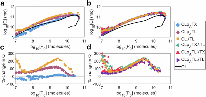
We consider an open-loop system (black) and six controllers: (a, c) CLpATX (blue), CLpATL (red), CLλTX (orange). b, d CLpATXλTL (teal), CLpATLλTX (crimson) and CLpATXλTL (purple). a, b Cumulative output Q against initial output P0. c,d Percentage-change in Q versus an open-loop system of equal initial output against initial output P0. Each marker represents a controller design from the multi-objective optimisation of P0, τ±10 and τ50. Simulation results are provided as a Source Data file.
The maximum cumulative protein production, Qmax, for each system is as follows: Open-loop, 1.42 × 10¹¹ mc; CLpATX, 1.54 × 10¹¹ mc; CLpATL, 1.59 × 10¹¹ mc; CLλTL, 2.47 × 10¹¹ mc; CLpATXλTL, 3.13 × 10¹¹ mc; CLpATLλTX, 2.46 × 10¹¹ mc; CLpATLλTL, 2.44 × 10¹¹ mc. Every controller is capable of enhancing the maximum possible cumulative output, even when Q has not been explicitly optimised for, with the best performing controllers having more than double the maximum cumulative open-loop output. All together these results suggest that the use of evolutionary stabilising negative feedback controllers has the potential to improve yields in industrial bioproduction settings.