
Our model of the AMC structure, illustrated in Fig. 1, consists of cylindrical nanowires connecting nearest-neighbor sites of a diamond lattice. Each nanowire has a length of l = 70 nm and a diameter d = 14 nm, resulting in a diamond-type AMC structure with a cubic lattice constant of ~162 nm.
Fig. 1: Three-dimensional nanowire array with a diamond-type structure.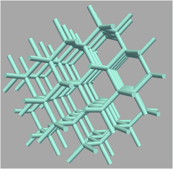
The array contains 238 nanowires and 155 vertices. Each wire has a length of 70 nm and a diameter of 14 nm. We assume an ideally soft-magnetic material with properties corresponding to those of typical FEBID-deposited nanoarchitectures11.
The magnetization in the artificial crystal exhibits the characteristics of a 3D ASI, as each wire is magnetized uniformly along its axis. This combination of two branches of research in magnetism—3D nanomagnetism and ASI—was recently discussed on the example of a buckyball-type geometry44. It is well known that the magnetization state of ASIs is not unique39,58. The lowest-energy arrangement of the magnetization is a defect-free magnetic configuration that satisfies the so-called ice rule at every vertex37, but ASI lattices can also contain several magnetic defect structures carrying monopole-type magnetostatic charges29,34,58.
Vertex charges and static configuration
Before addressing the magnetic high-frequency modes of the 3D array, it is instructive to analyze the possible micromagnetic configurations at the vertex sites, since—as we shall see—they have a decisive impact on the array’s dynamic properties. The diamond-type AMC has a coordination number of four: each vertex inside the 3D lattice is the intersection point of four nanowires. Regarding the coordination number, this type of lattice is therefore comparable to the well-known two-dimensional square ASI lattice32,43,59,60, which can be considered to be its two-dimensional (2D) counterpart. The main constituents of an ASI—in this case, the cylindrical nanowires—are usually of Ising type, meaning that their magnetic structure is homogeneous and aligned along the particle axis. The assembly of such Ising-type nanomagnets into a regular array can generate structures of varying complexity and magnetic frustration at the vertices. Vertex configurations in ASIs can be characterized by their magnetic charge44,58.
The definition of the vertex charge is based on the fact that—assuming Ising-type magnetization in each nanowire—each nanowire carries magnetic flux either toward the vertex or away from it. Any imbalance in the number of wires with in- and out-flowing magnetic flux results in a net magnetic charge at the vertex, akin to a magnetic monopole35,37,38. In the context of ASIs, such charged vertices are commonly referred to as magnetic defects, as they represent local violations of the ice rule and are associated with magnetostatic charges. With this premise, the charge of a vertex with coordination number four can take one of five possible values: +4q (“four-in”), +2q (“three-in/one-out”), 0, (“two-in/two-out”), −2q (“one-in/three-out”), and −4q (“four-out”). The value of the magnetic charge q can be estimated to q = r2πMs, where r is the nanowire radius and Ms is the saturation magnetization; a material-specific constant. Different vertex configurations and their resulting charges have been discussed in detail for 2D square ASI lattices40,61, and the same type of charge-based classification can also be made for vertex configurations in 3D diamond-type lattices. There is, however, a difference regarding the multiplicity of uncharged magnetic structures at the vertices in the 2D as compared to the 3D case. While in 2D lattices the zero-charge configuration exists in two different flavors61, it only appears in one form in the case of 3D diamond-type lattices (All zero-charge configurations in the tetrapod structure are equivalent as they can be mapped onto the one shown in Fig. 2a by means of a rotation and/or a time-inversion operation \(\vec{M}\to -\vec{M}\). Such a mapping is not possible for the different 2D variants in a square lattice shown in Fig. 2b, c). This reduction of complexity in the 3D system—compared to its 2D analog– simplifies the interpretation of the magnetic configuration in the diamond-type structure as it allows for identifying the vertex configurations uniquely by means of their charge, without the need to distinguish different flavors of zero-charge vertices.
Fig. 2: Zero-charge vertex configuration in a tetrapod structure—the elementary building block of a diamond-type 3D ASI lattice.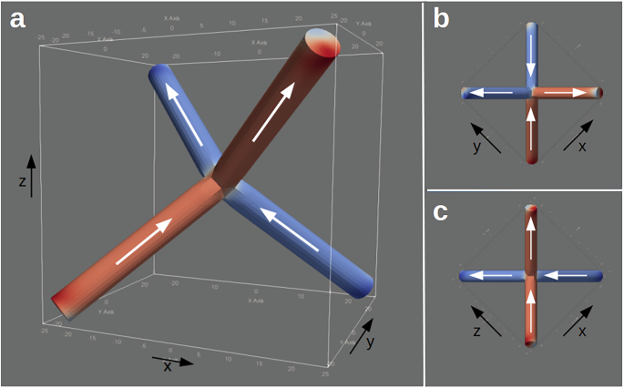
a Only one type of zero-charge configuration exists in 3D, whereas different zero-charge vertex structures are known from 2D square ice systems. The flavors of zero-charge vertex configurations shown in (b) and (c), known from 2D square ice ASI lattices, differ qualitatively in their micromagnetic structure, and they have different physical properties. Nevertheless, they can be interpreted as projections of a single 3D structure onto different planes. The color code represents the x-component of the magnetization.
Inside the 3D diamond-type ASI, each nanowire is connected to two vertices with even charges (±4q, ±2q, or 0). In addition to the vertices within the volume, a different type of charge exists at the lattice boundary (“surface”), where the wires are connected only to one vertex. The dangling ends of these outer nanowires can be considered as vertices with coordination number one and charge ±1q, where the sign indicates whether the magnetization points inwards or outwards. In total, the 3D diamond-type ASI lattice with Ising-type nanowires thus contains vertices of charges ±4q, ±2q, ±1q, and 0. Owing to time-inversion symmetry, the magnetic configurations of positive and negatively charged vertices are equivalent. It is therefore sufficient to distinguish the vertices only by their absolute charge, which effectively reduces the number of vertex configurations to four. In the diamond-type ASI lattice that we have studied, the diversity of vertex structures is further diminished by the fact that vertices with quadruple charges were never observed in the simulations, which indicates that these configurations are unstable. The magnetic state of the diamond-type ASI lattice is thus effectively characterized by the spatial distribution of double-charged defects of the type “three-in/one-out” and “one-in/three-out” (Fig. 3). A neutrality condition applies to the sum of vertex charges in the lattice, but not to the individual types: the presence of a double-charged vertex does not imply the formation of an additional double-charged vertex of opposite sign, so long as the sum of all vertex charges (including those at the surface) is zero.
Fig. 3: Different types of effective magnetic charges in the diamond-type 3D lattice.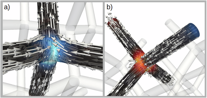
a Double-charge vertex with a “three-in/one-out” configuration, leading to an effective charge of +2. The orange colored region in (b) shows an equivalent “one-in/three-out” vertex with charge −2. The double-charge vertex in (b) connects two nanowires at the crystal surface whose dangling ends carry an effective charge of ±1. In both images, the color code displays the divergence of the magnetization. With this representation, the single charges appear as a weak orange and blue contrast near the ends of the wires at the top left and the top right, respectively. For better visibility, only a small subset of the computed magnetic moments is displayed with arrows.
The ice-rule-obeying zero-charge vertices are energetically optimal magnetic arrangements within the lattice, whereas charged vertex configurations are localized magnetic configurational defect structures, commonly referred to as magnetic defects in the ASI literature, increasing both the exchange and the magnetostatic energy. Defect charges within the AMC increase the magnetic disorder, which can be quantified by the density of charged vertices. In spite of their heightened energy compared to the defect-free state, magnetic structures containing several charged vertices can develop as metastable states, and they may persist even at sizeable external fields. Such multiplicity of metastable magnetization states is well known from 2D ASIs29,40 and similarly observed in our 3D diamond-type lattice. Removing defect configurations from the system requires external fields strong enough to magnetically saturate the sample, which is only achieved at fields exceeding ~100 mT.
Magnonic spectrum
To study the magnonic spectrum of the diamond-type AMC and how it is impacted by magnetic defects, we consider two different remanent magnetic configurations: a defect-free state, which will serve as the reference state, and a metastable state with random disorder. In the defect-free state, all vertices within the volume have the same two-in/two-out–type zero-charge configuration. Since the magnetic structure of the defect-free AMC is identical for each unit cell, the magnetic state shares the same periodicity as the crystal structure. The disordered state, on the other hand, contains several vertices with double-charge configurations (three-in/one-out or one-in/three-out), and its magnetic structure does not display any spatial periodicity. Double-charge vertices of different sign are randomly scattered within the AMC. In our case, the disordered state contains 35 double-charge vertices and 48 zero-charge vertices. This disordered state is only one realization out of a quasi-continuum of possible configurations39,62,63.
Let us first analyze the high-frequency modes developing in the ordered configuration. The magnonic spectrum of the defect-free configuration, shown in green (line a) in Fig. 4, displays five clearly defined peaks corresponding to distinct magnetic modes within the ASI lattice. Fourier analysis methods, through which the spatial distribution of the local oscillation amplitude (i.e., the mode profile) can be extracted for each frequency, reveal the central role played by the geometry in each of the peaks in the spectrum. Each of the prominent modes can be attributed to oscillations localized at different geometric constituents of the AMC–namely, the vertices in the volume, the cylindrical nanowires, and the wire ends at the crystal surface.
Fig. 4: Magnetic excitation spectrum of the ordered magnetic crystal and defect-induced modifications.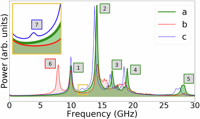
a Defect-free, ordered configuration: five distinct peaks appear, each corresponding to a different magnetic excitation. b Magnetic disorder introduces vertex defects, leading to an additional low-frequency mode \({\fbox{6}}\). The spectrum (c) refers to an AMC containing a structural defect site (missing nanowire).
The lowest-frequency mode at 9.9 GHz, denoted with the symbol \({\fbox{1}}\) in Fig. 4, is a surface contribution arising from the oscillations of the single-charge vertices on the outer shell. The color code used for the mode profile in Fig. 5a, b indicates inactive regions in purple color and maximum oscillation amplitude in yellow. Only the free ends of the single-connected wires partake in the magnetic oscillation at this frequency. This is the only surface contribution in the magnonic spectrum of the AMC. The relative height of the peak \({\fbox{1}}\) with respect to the other modes, therefore, depends on the crystal size and the resulting surface-to-volume ratio. The oscillations at the wire ends appear to be decoupled from one another. No clear correlation is observed among the phases of this oscillation at different sites (see Movie 1 in the supplemental material).
Fig. 5: Fundamental modes of the defect-free diamond-type AMC.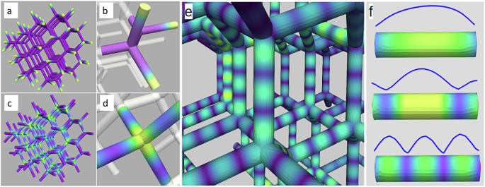
The low-frequency modes, corresponding to the peaks labeled \({\fbox{1}}\) and \({\fbox{2}}\) in Fig. 4, are oscillations localized at the surface and volume vertices, respectively. a The mode at 9.9 GHz refers to oscillations of the free ends, i.e., to the outermost vertices at the crystal surface, as shown in the magnified view in frame (b). The strongest excitation in the spectrum, displayed in frame (c), is due to vertices within the volume which become active at 14.2 GHz. The magnified view (d) shows the localization of the mode at the vertex sites. e The high-frequency modes at 16.7 GHz, 19.1 GHz, and 28.2 GHz (corresponding to the peaks \({\fbox{3}}\), \({\fbox{4}}\), and \({\fbox{5}}\), respectively) are oscillations describing longitudinal standing spin waves in the nanowires. Frame (f) shows the computed mode profile along the nanowires for these standing-wave modes, with frequency increasing from the top to the bottom. In all panels, the color code ranging from purple to yellow describes regions of minimum and maximum oscillation amplitude, respectively.
The most pronounced peak in the spectrum develops at 14.1 GHz (see label \({\fbox{2}}\) in Fig. 4). The corresponding mode is an oscillation of the magnetization at the zero-charge vertices within the array. The profile of this mode, shown in Fig. 5c, d, displays a clear localization at the center of the tetrapod-shaped vertices. Only the vertices within the volume are active; the free ends do not oscillate at this frequency. Contrary to the mode localized at the free ends at the surface, the oscillation phases of the individual vertices are strongly correlated and nearly synchronous throughout the volume (see Movie 2 in the supplemental material).
Three distinct high-frequency peaks can be identified in the spectrum of Fig. 4, labeled \({\fbox{3}}\), \({\fbox{4}}\), and \({\fbox{5}}\). At these frequencies, standing waves develop in the nanowires. Figure 5e shows the mode at 28.2 GHz, in which the magnetic oscillation within each wire contains four nodes and three anti-nodes. The profiles of this category of modes are displayed in Fig. 5f). In this figure, the wires have been shown isolated from the main crystal for clarity, although they remain magnetically and structurally embedded into the AMC. In these standing-wave modes, remarkably, the wire ends (i.e., the vertices) neither act as free nor as fixed ends of the oscillation. At 16.7 GHz and 28.2 GHz, the vertices remain inactive, while at 19.1 GHz the magnetization also oscillates at the vertices. Although there appears to be a certain phase correlation of the standing-wave modes in different wires within the crystal, it is not always as clear as in the case of the vertex mode \({\fbox{2}}\). The modes can be viewed in the movies 3–5 of the supplemental material. A clear macroscopic correlation can be observed only for mode \({\fbox{4}}\), which is the only one where the volume vertices participate in the oscillation. This suggests that long-range dynamic correlations primarily result from the dynamic interaction between the volume vertices.
Modes in the magnetically disordered state
Up to this point, we have investigated the magnetic high-frequency modes of an AMC in which the structure is magnetically ordered, such that all vertices in the volume have a zero-charge magnetic configuration. Although the magnetic structure is inhomogeneous (there are six different magnetization directions in the nanowires, according to their orientation in space), the magnetic modes do not appear to be influenced by the magnetic structure. The modes discussed so far appear to be tightly connected to the structural or geometric elements of the AMC: vertices, nanowires, and surface, not to the magnetization.
A strong influence of the magnetic structure on the high-frequency spectrum, however, is revealed when analyzing the magnetically disordered AMC. The excitation spectrum of the disordered state, shown in red in Fig. 4 (line b), displays significant differences with respect to that of the ordered AMC (line a). The most striking change is the appearance of an additional low-frequency mode \({\fbox{6}}\) at 7.9 GHz. This mode corresponds to oscillations localized at the double-charge vertices (three-in/one-out and one-in/three-out configurations), which are present in the ordered state but absent in the ordered one. The appearance of this mode is a clear example of a spectral feature that is directly governed by the magnetic configuration. Interestingly, the zero-charge vertices \({\fbox{2}}\) that persist in the disordered AMC oscillate at a frequency markedly different from that of the double-charge vertices, even though they are localized at identical geometrical sites.
The oscillation profiles of the zero-charge and double-charge vertices, shown in Fig. 6a, b, respectively, are complementary. Only double-charge vertices are active at 7.9 GHz, and only zero-charge vertices participate in the mode at 14.2 GHz. In spite of this clear separation in terms of frequency and micromagnetic configuration, the oscillation amplitude of the different vertices is not identical within each of these modes. Some vertices display strong oscillations, whereas a few vertices show only little activity. We attribute this inhomogeneity in amplitude to local variations in the internal magnetic fields, arising from the magnetostatic influence of nearby charged vertices. The frequency of the zero-charge vertices and the local mode profile of the active vertices remain mostly the same as in the ordered AMC, but the phase correlation between the vertices is lost in the disordered state (see Movie 6 of the supplemental material). Compared with the ordered case, the intensity of the zero-charge vertex mode \({\fbox{2}}\) is reduced in the disordered state, in accordance with the lower density of this type of vertex in the disordered AMC.
Fig. 6: Vertex modes in the disordered state.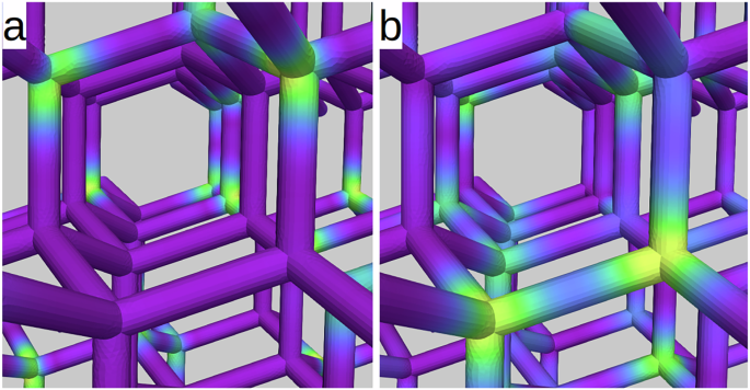
Frame a shows the mode profile at 14.2 GHz. Only the vertices with a zero-charge type magnetic configuration partake in the oscillation at that frequency. The frequency as well as the local mode profile of the oscillating zero-charge vertices are the same as in the ordered state, shown in Fig. 5c, d. The vertices with a double-charge configuration are active at a significantly lower frequency (7.9 GHz). The mode profile of this oscillation, shown in frame (b), highlights the activity of a set of vertices that is complementary to that in the mode shown in frame (a).
A more significant difference between the ordered and the disordered spectra concerns the peaks \({\fbox{3}}\) and \({\fbox{4}}\) describing the first and the second standing-spin-wave modes in the nanowires. In the disordered AMC, these peaks significantly broaden and become almost indiscernible. Instead of the two well-defined peaks, a weakly defined quasi-continuum of overlapping modes appears in the frequency range between 15 and 19 GHz. A detailed Fourier analysis of the individual nanowires shows that these modes are still present in the disordered crystal. However, their frequencies now differ from one nanowire to another, resulting in a broadened and blurred spectrum in this frequency range. This effect, too, is attributed to the spatial variation of local magnetic fields arising in the disordered state. Charged vertices generate local magnetic fields within the disordered crystal that are absent in the ordered state. The magnetic divergences developing, for example, in a vertex with a negative double charge (three-in/one-out configuration) and those in a positive double-charge vertex (one-in/three-out) are monopole-type sources and sinks of the magnetic field \(\vec{H}\), respectively. Correspondingly, a longitudinal magnetic field develops in a nanowire, forming a Dirac string27 that connects two such vertices of opposite charges35,43. Such longitudinal magnetic fields result in a shift of the standing-wave modes to different frequencies64.
There are numerous possible combinations of vertices that can be pairwise connected by a nanowire in the disordered state, since vertices can differ in both magnitude and sign of the magnetic charge they carry. Accordingly, although the homogeneous and axial magnetization structure is the same in all nanowires, their high-frequency magnetic dynamic properties differ as a result of a broad distribution of local fields throughout the crystal. In addition to differences in magnitude, the magnetic field developing in wires connecting oppositely charged vertices can also differ in sign. The dipolar magnetic field generated by the vertex charges can be parallel or antiparallel to the wire magnetization. This leads to two qualitatively different cases, resulting in an additional lift of the degeneracy of nanowire modes.
Compared to the modes \({\fbox{4}}\) and \({\fbox{5}}\), the higher-frequency excitation \({\fbox{6}}\) at 28 GHz remains largely unaffected by the magnetic disorder of the crystal. In general, high-frequency modes are dominated by the exchange interaction, which leads to local effective fields that are much larger than those due to dipolar fields. Correspondingly, changes in the dipolar field distribution have a weaker impact on exchange-dominated high-frequency modes.
Impact of structural defects
Having established that charged vertices, which represent magnetic defects, strongly affect the high-frequency properties of the AMC, we now analyze how a structural defect changes the magnetic spectrum. We introduce a structural defect by removing a single nanowire inside the AMC, as shown in Fig. 7a. This removal results in two defect vertices with reduced coordination number as they represent the junction of three instead of four nanowires. To isolate the effect of this structural defect on the high-frequency properties of the AMC, it is introduced as a modification of the otherwise defect-free magnetic state, i.e., the ordered reference state. Despite obeying the spin-ice rule, both defect vertices carry a magnetic charge due to their two-in/out-out and one-in/two-out configurations. These result in charges of ±1q, while preserving the overall charge neutrality of the AMC.
Fig. 7: Structural defect within the AMC giving rise to an additional mode localized at the defect site.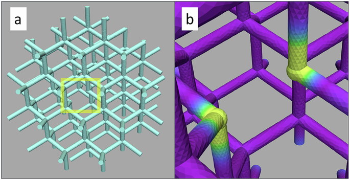
a Shows the modified AMC in which a single nanowire has been removed. The removal of a nanowire introduces two vertices with reduced coordination number, which oscillate at 11.7 GHz. The spatial distribution of this mode is localized at the defect site (b). This defect mode appears in the spectrum as a small peak labeled \({\fbox{7}}\) in the inset of Fig. 4.
Although the magnitude of these charges equals that of surface vertices, the defect vertices are different in terms of their magnetic structure and charge type. They carry volume-type magnetostatic charges, while the free ends have surface-type charges65. The magnonic spectrum of the AMC with a structural defect [represented as a line in Fig. 4c] demonstrates the appearance of an additional, weakly pronounced mode (label \({\fbox{7}}\) in the inset). As shown in Fig. 7b, this mode is localized at the defect vertices. It has a low intensity in the spectrum because the signal originates from only two defect vertices out of a total of more than 100 surface and volume vertices in the AMC. This localized mode could serve as a spectral fingerprint for identifying or characterizing structural defects in experimental realizations of AMC systems. Besides this additional low-amplitude peak, the introduction of a structural defect also leads to a clear shift of the volume modes \({\fbox{3}}\), \({\fbox{4}}\), and \({\fbox{5}}\) toward lower frequencies. Adding more structural defects exacerbates this effect and leads to further changes in the spectrum. As the number of structural defects increases, their influence can no longer be treated as a perturbation to the defect-free state, and the resulting spectral modifications become substantial.
Field dependence of magnonic spectra
To further characterize the magnonic properties of the AMC, we investigate how the magnetic absorption spectra evolve under an external magnetic field. We focus on the field dependence of the spectrum of the ordered configuration in Fig. 4a, corresponding to the defect-free configuration. This state is achieved by quasi-statically reducing an external field from saturation to zero. The field is initially applied along the z direction of the AMC (cf. Fig. 2), such that each of the four sets of nanowires encloses the same angle with the applied field. We refer to this orientation as the “parallel” case, in contrast to the “perpendicular” case, where the field is applied orthogonally to the z axis, i.e., to the remanent magnetization direction. In both configurations, we vary the field strength in a range of 200 mT. For each field value, we compute the static magnetization structure and its oscillatory small-amplitude dynamic response. The resulting spectra for the parallel and perpendicular cases are shown in Fig. 8a, b, respectively. The results are obtained using a recently developed numerical method66, specifically designed to simulate such situations. The color scale indicates the absorbed power as a function of frequency and field strength, with the zero-field line reproducing the four lowest-frequency peaks seen in Fig. 4a)
Fig. 8: Field dependence of magnonic absorption in the defect-free, high-remanence configuration.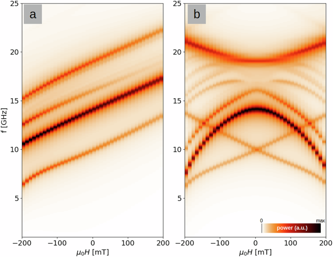
The spectra evolve differently depending on the orientation of the applied magnetic field relative to the remanent magnetization: a shows the case of a parallel field, whereas b corresponds to a perpendicular field.
In the parallel case [Fig. 8a], the resonance frequencies vary approximately linearly with the applied field, with a slope of ~18 GHz T−1. Over the considered range, the intensities of the individual resonances remain nearly constant, except for the third peak (denoted as \({\fbox{3}}\) in Fig. 4 and identified as the first standing-wave mode within the nanowires), whose intensity decreases with positive and increases with negative field strength.
In contrast, the perpendicular-field case [Fig. 8b] shows markedly different behavior. The resulting magnonic absorption spectrum is symmetric about H = 0 and exhibits several notable features. The lowest-frequency mode \({\fbox{1}}\), associated with oscillations of the free ends at the surfaces, shows a clear Zeeman-type splitting. Other modes display more complex field dependencies, with some increasing and others decreasing in frequency as the absolute field strength grows. At higher fields (∣μ0Hext∣ > 100 mT), additional absorption lines appear–some of which appear to branch from the second-order standing spin-wave mode \({\fbox{4}}\).
These findings demonstrate that the field-dependent absorption spectra of the AMC are strongly anisotropic: an external field can modify the spectrum very differently depending on whether it is applied perpendicular or parallel to the remanence direction. This behavior resembles that reported for ASI systems under field67, and suggests the potential for using AMCs as reconfigurable magnonic platforms with tunable spectral properties.