
Collecting and processing of field A. thaliana leaf samples
We shared most parts of the sampling trip with those of ref. 10. We took samples from the same 12 sites across Sweden, Spain, France, and replaced three sites from Northern Germany to three sites near Tübingen, Germany (Supplementary Table 6). We harvested A. thaliana from February to May at the same developmental stage (bolting/flowering stage) for one (one site), two (one site) and three (13 sites) consecutive years. Using sterilized tweezers, whole leaf samples were prepared by roughly cleaning the leaves of dirt, inserting them into 2 ml tubes and storing the tubes immediately in dry ice. The endophytic samples were instead prepared by subjecting leaves to surface sterilization. The rosette was surface sterilized by washing with 80% ethanol for 15 s, followed by 2% bleach (sodium hypochlorite) for 30 s. Rosettes were rinsed three times with sterile autoclaved water for 10 s before being placed in a screw-cap tube and frozen on dry ice as endophytic samples. All samples were shipped to the Max Planck Institute for Plant Breeding Research in Cologne (Germany) and stored at −80 °C until further processing. We took 6–10 plants from each site, with half processed as whole leaves and the other half as endophytes. In total, 347 samples were collected.
DNA extraction from field samples and amplicon library preparation
DNA extraction and library preparation of all field samples were carried out with the same previously described method17. Briefly, 0.2 g acid-washed and sterilized zirconium beads at different sizes (0.1–0.5 mm diameter) and 500 μl DNA extraction buffer were added to plant samples. The buffer consisted of 0.5% SDS, 50 mM Tris buffer at pH 8, 200 mM NaCl, 2 mM EDTA, 1 mg ml−1 lysozyme and 100 mg ml−1 proteinase K. The samples/beads were first incubated for 45 min at 37 °C, and were then beaten using a Bertin Precellys 24 (Bertin Technologies) at 6,300 r.p.m. for 2 × 45 s with a 15 s pause. A second incubation was then carried out at 37 °C for 45 min in the presence of 10 µg ml−1 RNAse. The tubes were then centrifuged at 10,000 r.p.m. for 2 min and the liquid was transferred to a new tube. The nucleic acids were cleaned up with 600 μl phenol/chloroform/isoamyl alcohol (25:24:1) and chloroform/isoamyl alcohol (24:1), then precipitated by adding 0.1× of the sample volume of 3 M sodium acetate and 1,500 μl 100% ethanol and centrifuging at 4 °C at 15,000 r.p.m. for 40 min. The product was washed twice with 70% ethanol and eluted with 30 μl 10 mM Tris buffer pH 8.0. To avoid potential problems with PCR inhibition, samples were mixed 1:1 with 20% Chelex-100 and allowed a 30-min contact time, after which the liquid fraction was recovered and stored at −20 °C until further use.
PCR amplification was performed in two steps to allow the use of blocking primers to decrease plant plastid contamination that occurs with 16S amplification. The samples were diluted with 10 mM Tris HCl to 50 ng μl−1 before being used in the first PCR step. In the first step, universal primers and blocking oligos (Supplementary Table 7) were used together to amplify targeted regions. For each target taxonomic group, two universal primer pairs were used. Each of the 20 μl reactions contained 0.2 μl Q5 high-fidelity DNA polymerase (New England Biolabs (NEB)), 4 μl Q5 High-GC buffer, 4 μl Q5 5× reaction buffer, 0.16 μl of each forward and reverse primer (10 μM), 0.5 μl of each blocking primer, 0.5 μl dNTPs (10 μM), 1 μl template DNA and nuclease-free water to a final volume of 20 μl. Triplicates were run in parallel on 3 independent thermocyclers (Bio-Rad); cycling conditions were 95 °C for 40 s, 10 cycles of 95 °C for 35 s, 55 °C for 45 s, 72 °C for 15 s, and a final elongation at 72 °C for 3 min. The 3 reactions were combined and 10 μl were used for enzymatic cleanup with Antarctic phosphatase and Exonuclease I (NEB; 0.5 μl of each enzyme with 1.22 μl Antarctic phosphatase buffer at 37 °C for 30 min followed by 80 °C for 15 min). The second step of PCR was carried out in a single 50 μl reaction. The reaction included: 0.5 μl Q5 DNA polymerase (NEB), 10 μl Q5 High-GC buffer, 10 μl Q5 5× buffer, 1 μl dNTPs (10 μM), 0.83 μl of each barcoded primer (10 μM) and 26.34 μl nuclease-free water. A volume of 0.5 μl of the cleaned-up first-step PCR product was added to each reaction. The protocol used in the thermocycler was: 95 °C for 40 s, followed by 25 cycles of 95 °C for 35 s, 55 °C for 45 s, 72 °C for 15 s, and 72 °C for 2 min. The barcoded amplicons were then cleaned using AmPure XP beads (Beckman-Coulter) following manufacturer protocol. Magnetic beads solution (40 μl) was added to the 50 μl barcoding reaction, shaken for 5 min at 700 r.p.m. at room temperature, then washed twice with 200 μl 80% ethanol, dried and resuspended in 25 μl 10 mM Tris. Amplicons were quantified in duplicates with the PicoGreen system (Thermo Fisher) and samples were combined in equimolar amounts into one library to reach 8 pmol per library. The final libraries were also cleaned with 0.8× volume AmPure XP purification beads and eluted into 40 μl. Libraries were prepared with the MiSeq Reagent Kit v.3 for 2 × 300 bp paired-end reads (Illumina) with 3% PhiX control. Quality assessment and the eventual presence of contaminants were assessed using a bioanalyzer (Agilent). The final concentration of the pooled libraries was finally assessed using a Quantus Fluorometer (Promega) following the indications of the manufacturer. Since there is a maximum of 50 barcoded primers per locus available, we performed 8 runs in total to cover all the samples. The sequencing libraries were run by the Illumina MiSeq platform in house.
Amplicon data processing and OTU table filtering
The detailed steps for raw amplicon data processing are summarized in Supplementary Information, with all scripts available at Amplicon_data_analysis/Amplicon_sequencing_processing60. The raw OTU tables for each taxonomic group were exported from QIIME (v.2023-07)61 and were handled with Python. We first chose the amplicon with the highest number of classified OTUs from each taxon group for further filtering. We next applied several modification steps sequentially: (1) filtering of OTUs that do not belong to the corresponding taxonomic group (for example, non-bacterial OTUs within the BacV5 amplicon); (2) merging all OTU tables from each taxonomic group; (3) filtering of OTUs with fewer than 50 counts and present in only one sample; (4) separating OTU tables by compartment: whole leaf and endophytes; (5) selection of the amplicon with higher number of classified taxa to proceed further for each taxonomic group; (6) normalizing the count of each OTU to the total count of its corresponding taxonomic group of each sample, and calculating the relative abundance; and (7) selection of the samples containing OTUs from all four taxonomic groups. The detailed Python script for this step is available under Amplicon_data_analysis/OTU_table_processing/filter_otu_and_tax_final.ipynb60. The final OTU tables were deposited in Amplicon_data_analysis/OTU_table_processing/processed_OTU_tables.
Diversity analysis
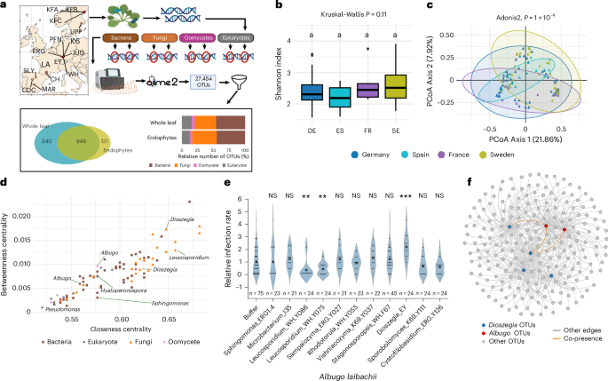
On the basis of the final OTU table, we calculated the Shannon index using the R package vegan62 and grouped the OTUs by country of origin for comparison. To control for potential bias introduced by varying sample sizes across different countries, we subsampled the reads from each sample 100 times and conducted Kruskal–Wallis tests for each iteration. We only observed 10 of the 100-times subsampled reads, showing significant differences in the Shannon index across the four countries, supporting the idea that the results without subsampling are unbiased.
For analysing beta diversity, distance matrices using Bray–Curtis distance were calculated for all samples and the subsets of whole-leaf and endophytic samples using the R packages vegan and ade4 (ref. 63). Plotting of the results and statistical testing using permutational multivariate analysis of variance (PERMANOVA) were conducted with the first and second principal components using ggplot2. For PERMANOVA analysis, all groups were compared at once for both endophyte and whole-leaf plots using the PERMANOVA function in the vegan R package.
To identify the most occurring taxa from each country, we calculated the relative abundance of the 10 most abundant classes for bacteria, fungi and other eukaryotes. For oomycetes, we calculated the 10 most abundant genera since all samples only contain one (endophytes) or two (whole leaf) oomycete classes. We used the phyloseq package64 for this analysis. Samples were first merged by country and subsequently normalized to relative abundance, and OTUs with an undetermined class were grouped in the category ‘unassigned’. All classes with lower abundances than those categorized in the top 10 were grouped into the category ‘other.’ Subsequently, the average relative abundances were plotted using ggplot2 (ref. 65).
All R scripts for analysis and figure plotting are summarized in Amplicon_data_analysis/diversity_analysis.
Network analysis
Before network construction, the OTU table was filtered to only contain OTUs present in 10 or more samples to retain the most conserved taxa among all samples. The subsequent network construction was performed using Fastspar24, using the recommended settings for bootstrapping and permutation counts. The resulting P value and median correlation tables were transformed into an edge table using R, keeping all interactions with a P value lower than 0.1 and a none-zero value. We selected this relatively loose thresholds since we have applied strict filtering for the most conserved OTUs, so we wanted to retain most of their interactions including the weak interactions. We used the built-in function of the network analyser Cytoscape (v.3.9.1)66 to calculate degree, betweenness centrality and closeness centrality, and the final visualizations of the networks were constructed utilizing Gephi (v.0.10.1)67. The script for constructing the network is available at Amplicon_data_analysis/Network_analysis_and_Albugo-Dioszegia_interaction60.
Microbial growth conditions
All microbial strains used in this study are summarized in Supplementary Table 2. All fungi used were grown on potato dextrose agar (Carl Roth) and bacteria in nutrient broth agar (Carl Roth). The spore collection and inoculation of the Albugo laibachii was performed according to ref. 19. Briefly, infected leaves with clear white pustules were collected and resuspended in Milli-Q water in 50 ml tubes. The tubes were incubated on ice for 1 h, and the spore suspension was filtered with a 40 μm filter (Greiner Bio-One). The spore suspension was then sprayed on plants using a spray gun with an air pump, and plants were incubated at 8 °C in the dark overnight. Infected plants were kept under 8-h light and 16-h dark cycles, a 20 °C day and 16 °C night temperature, and 60% humidity for 14 days or until infection symptoms appeared.
Gnotobiotic microbial inoculation on A. thaliana
The gnotobiotic microbial inoculation system was adapted from refs. 68,69 with some modifications. Briefly, A. thaliana ws-0 (Wassilewskija) seeds were sterilized for 6–12 h with chlorine gas. Sterilized seeds were immediately sown on 0.5× Murashige and Skoog (MS) with 0.75% agar and incubated under 8/16-h light/dark cycles with a 20 °C day and 16 °C night temperature, and 60% humidity. After 7 days, the germinated seedlings were placed onto 12-well plates (Greiner Bio-One) with each well filled with 2.5 ml 0.5× MS agar. Plates with seedlings were further incubated for 3 weeks before spraying.
We primarily tested fungi (yeasts) and few bacteria in this study, either because isolation of the predicted Albugo-interacting bacteria was unsuccessful or these are slow growers (actinobacteria) and therefore not compatible with co-inoculation with Albugo. To spray different bacteria and fungal strains, we directly streaked fresh bacteria or yeast colonies (<5-day growth) from agar plates and resuspended them in 10 mM MgCl2 solution. We then diluted the strain resuspensions to reach optical density at 600 nm (OD600) of 0.5. To spray Fusarium and Stagonosporopsis strains, 10 ml 10 mM MgCl2 was added into each plate that was fully covered with fungal mycelium and spores (>14-day growth). We then used a 1 ml pipette tip to streak the plate and release a maximum number of spores, which were filtered with a 40 μm filter (Greiner Bio-One). We then counted the spores with a haemocytometer and diluted the spores to reach 104–105 spores per ml. After dilution, all microbial solutions were transferred into airbrush guns (Conrad Electronics) and sprayed two times (~40 μl each) with the air pump (Conrad Electronics) at 0.5 bar pressure. After spraying buffer and different microbial strains, we waited 2–3 h to allow the evaporation of excess water before spraying A. laibachii. To minimize the effect of A. laibachii spore-associated microbes and ensure a gnotobiotic infection environment, we treated the A. laibachii spores with antibiotics. We first incubated the Albugo-infected leaves with autoclaved Milli-Q water on ice for 1 h to facilitate the release and hatching of A. laibachii sporangia (one full 50 ml tube of infected leaves filling up with water). The spore solution was then filtered with a 40 μm filter (Greiner Bio-One) and centrifuged at 4,000 g in 15 ml tubes for 10 min at room temperature. We next removed the supernatant and resuspended the spore pellet gently with a 5 ml antibiotic solution containing 2.5 mg kanamycin, streptomycin and rifampicin, plus 1.25 mg geneticin. We incubated the spores with the antibiotic solution at room temperature for 25 min in the dark, before pelleting again by centrifuging the tube at 4,000 g for 10 min. The supernatant was removed and the antibiotic-treated spores were washed twice with autoclaved Milli-Q water and once with 10 mM MgCl2 using the same centrifugation conditions. The antibiotic-treated spores were resuspended with 10 mM MgCl2 and adjusted to 106–107 spores per ml before spraying on the sterile plants using the same airbrush setup as for other microbes. After spraying the A. laibachii, all 12-well plates were sealed with a breathable tape and bagged with transparent bags to keep the humidity at >90%. The bagged plates were incubated at 8 °C in the dark overnight before transferring to the growth chambers. The transparent bag was removed after another day (day 2). The infected plants were scored and harvested for qPCR at 12 dai.
Quantification of Albugo in planta with scoring and qPCR
To score infected plants from gnotobiotic infection systems, we first removed all root tissue of each plant and recorded the number of infected leaves for each plant. We then divided the total number of infected leaves by the total number of plants from each treatment group to calculate the average number of infected leaves per plant (ANIL). Since the efficacy of A. laibachii infection varies considerably among individual plants, we tried to ensure the robustness of the experiment by only including results from experiments with 0.5–2 ANIL in the control group (buffer and A. laibachii). The A. laibachii infection was considered unsuccessful if the ANIL was below 0.5. In addition, the difference between buffer and treatment groups cannot be observed if the infection is too good (ANIL > 2.5), since there were only 4–5 mature leaves in total when A. thaliana plants were sprayed. To control for the impact of zeros in statistical analysis and balance results from experiments with varied infection levels, we also added a pseudo-count (0.05) to all scoring data before calculating the ANIL.
After scoring, the rosette was put into 50 ml falcon tubes and divided into 3–6 groups as biological replicates with 3–5 plants per group for DNA extraction and qPCR. The rosette tissues were snap frozen in liquid nitrogen and ground with mortars and pestles. We used the silica column-based DNeasy plant mini kit (Qiagen) following manufacturer protocol. DNA concentration was measured with a NanoDrop spectrophotometer (Thermo Fisher) and adjusted to 5 ng μl−1 with Milli-Q water before processing for the qPCR experiment. We used SsoAdvanced Universal SYBR Green Supermix and a CFX Connect real-time PCR detection system (Bio-Rad) for qPCR reaction following manufacturer instructions. We used 20 μl reactions and 5 μl (25 ng) DNA as template. For each sample, we performed two reactions for the EF1α genes of both A. laibachii and A. thaliana. Quantification cycle (Cq) values obtained from A. laibachii DNA amplification were first normalized to A. thaliana DNA amplicon from the same sample using the formula \({2}^{-\Delta {C}_{q}}\) to calculate the relative A. laibachii quantity per sample. Then the relative Albugo quantities of each treatment sample were normalized to the average relative Albugo quantity of the buffer control to compare among different experiments. Each data point in the figure represents 3 technical replicates.
ELISA assay
To measure the secretion of thiamine, Dioszegia strains (EY, PT, EYΔper1 and the complemented strain) were cultured in thiamine-free Yeast Nitrogen Base (YNB) medium (FORMEDIUM) supplemented with 1% glucose and a complete set of amino acids (FORMEDIUM). After 3 days, the cultures were collected and filtered through a 0.2 μm filter to separate the extracellular fraction from the yeast cells. The resulting cell-free supernatants were analysed immediately using a competitive Vitamin B1 (Thiamine) ELISA kit (Abbexa, abx150384) following manufacturer instructions.
Briefly, 50 μl of the filtered samples or thiamine standards (ranging from 3.7 ng ml−1 to 300 ng ml−1) were added to a 96-well microplate pre-coated with a thiamine-specific antibody. Biotin-conjugated Detection Reagent A (50 μl) was added to each well, and the plate was incubated for 1 h at 37 °C. Following incubation, the plate was washed three times with 1× Wash Buffer to remove unbound components. Subsequently, 100 μl of HRP-conjugated Detection Reagent B was added to each well and incubated for 30 min at 37 °C. After a second washing step (5 times), 90 μl of TMB substrate was added and incubated at 37 °C for 5 min in the dark. The reaction was terminated by adding 50 μl of Stop Solution.
Optical density was measured at 450 nm using a microplate reader. Thiamine concentrations were calculated by plotting the OD values against a standard curve. The raw data and the standard curve were deposited in the Gitlab repository at /Scripts_for_data_analysis_and_figure_plotitng/scripts_for_figure_ploting/ELISA_data.xlsx60.
Dioszegia genome information
The detailed DNA extraction, sequencing, assembly and annotation steps are summarized in Supplementary Information. All sequenced strains and the quality assessment of assemblies are summarized in Supplementary Table 3. All raw data were submitted to NCBI Sequence Read Archive (SRA) under the BioProject PRJNA1190083. All genome assemblies were submitted to GenBank and the accession number for each genome is recorded in Supplementary Table 3. Copies of the assemblies, gene predictions and functional annotation used in this project were posted at /Supplementary_files/Dioszegia_genomes_and_annotations/. Detailed scripts used for all above steps are available at /Scripts_for_data_analysis_and_figure_plotting/Genome_analysis.
Extraction of thiamine metabolism genes and cloning of DhPER1 orthologues in different Dioszegia strains
We manually inspected the functional annotation result of Dioszegia EY and PT genomes and extracted the thiamine metabolism genes by searching the keyword ‘thiamine’ in the functional annotation file. In total, 14 genes were identified from each genome. We paired these genes through alignment and validated them by Sanger sequencing in case the paired genes were predicted to be substantially different in gene size (>10%) or exon borders. After Sanger sequencing validation, all alleles ended up with a similar size and were translated to amino acid (AA) sequence for alignment. The CDS and AA sequence were then aligned to calculate the SNPs per kilobasepair and variations per 100 amino acids.
To search for genes homologous to DhPER1 from different Dioszegia strains, we used two strategies. First, we searched different parts of DhPER1 in all available Dioszegia genome assemblies from both online databases and in-house sequencing using Geneious Prime v.2024.0.5 (https://www.geneious.com). We found six DhPER1 homologous genes using this method. However, we did not find the DhPER1 paralogue from the nanopore assembly of Dioszegia Y22 strain. Therefore, we performed a PCR test using the DhPER1 primers, and the PCR test resulted in the identification of the Y22 paralogue of DhPER1. This result also indicated that the nanopore assembly was largely inaccurate for this strain, hence we performed the Illumina sequencing and assembly again for Y22 (Supplementary Table 3).
RNA-seq experiments and data analysis
We performed two RNA-seq experiments. The first is the analysis of Dioszegia EY and PT transcriptome to validate the expression profile of DhPER1 in vitro. The second experiment is the RNA-seq analysis of A. laibachii and D. hungarica inoculated on sterile A. thaliana leaves at 2 dai. For both experiments, the RNeasy plant mini kit (Qiagen) was used for RNA extraction, and the Turbo DNA-free kit (Thermo Fisher) was used for the removal of the remaining DNA. The purified RNA was then quality controlled by agarose gel electrophoresis and bioanalyzer (Agilent) using the corresponding RNA kit before sending to BMKGene for sequencing.
We performed PacBio long-read RNA sequencing (IsoSeq) for the D. hungarica comparative transcriptomics experiment, with one sample for each strain. The circular consensus (CCS) reads from Dioszegia EY and PT were received and mapped to their corresponding DhPER1 paralogues using Geneious RNA mapper and visualized within Geneious Prime (v.2024.0.5). The raw CCS reads from EY and PT were deposited at NCBI SRA under accession ID SRR31480791 and SRR31480792.
For the RNA-seq data from Albugo- and Dioszegia-inoculated sterile A. thaliana at 2 dai, we used Illumina sequencing and performed three biological replicates for each of the three treatment groups (Albugo, Albugo + EY, Albugo + PT). We used a standard RNA-seq analysis workflow70 to analyse the data from each treatment group separately. First, the raw Illumina fastq data were quality controlled with FastQC71 before trimming with fastp (v.0.24.0)72. We then concatenated the genome assembly, transcripts and annotation files of A. thaliana (TAIR10)73 and A. laibachii19 before mapping the quality-controlled fastq reads to it with HISAT2 (2.2.0) using default parameters74. We assembled the mapped reads into transcripts and calculated the fragments per kilobase of transcript per million read pairs (FPKM) and transcripts per million (TPM) for A. thaliana and Albugo genes using StringTie (2.2.0) with default parameters75. Principal component analysis (PCA) was performed on the FPKM of each sample. Similarity among samples was displayed by reducing dimensionality into two or three principal components. Then, we used the ggplot2 R package65 for visualizing the PCA of the two most related components. We next used DESeq2 (ref. 76) to investigate the differentially expressed Albugo genes induced by D. hungarica. The list of differentially expressed Albugo genes was extracted and submitted to ShinyGO (v.0.82)77 for the GO analysis with an FDR cut-off of 0.05 and 4 genes per group selection criteria. The Illumina RNA-seq data were deposited at NCBI SRA under the following accession IDs: SRR31531712–SRR31531717 and SRR31512421–SRR31512423. The intermediate HISAT2 and StringTie output files and main scripts used in this step are available at Scripts_for_data_analysis_and_figure_plotting/RNAseq_DEG_analysis/60.
Structure modelling of DhPER1 and molecular docking
Structure predictions were conducted with AlphaFold2 (v.2.3.0)78 using the full databases for multiple sequence alignment (MSA) construction. We produced five models and selected the best model for visualization purposes. The structure of the yeast thiamine permease THI7 was downloaded from UniProt79. Structures of all permeases (.pdb files) and molecular docking files (.sdf) were posted at /Supplementary_files/Permease structure prediction/. We used PyMOL80 for visualization of structures.
Gene cloning and plasmid construction
We used three plasmids in this study, and they were all amplified in E. coli DH5α strain. The CRISPR plasmid (pHSP:CRISPR) contains a high-fidelity variant codon optimized Cas9 gene for Ustilago maydis81. The single guide RNA (sgRNA) was designed using Geneious Prime (v.2024.0.5) and we chose the target close to the 5’ end of DhPER1. The plasmid pHSP:CRISPR was linearized with restriction enzyme Acc65I and assembled with sgRNA oligo and ‘scaffold RNA’ fragment with 3’ downstream 20 bp overlap to the plasmid using Gibson Assembly (NEB) following manufacturer protocol.
The hygromycin resistance gene (HygR) and DhPER1-expressing vectors were generated using a shuttle vector EC35 from the fungal Golden Gate system developed for Ustilago maydis as backbone82. To construct the HygR-expressing vector pHSP:HygR, EC35 was first digested with BamHI and XbaI (NEB), and the HSP::HygR cassette was amplified from the pHSP:CRISPR vector using primer YH67 and YH55. The two fragments were assembled together using Gibson Assembly (NEB) following manufacturer protocol. To generate the pHSP:PER plasmid, we first amplified the HSP70 promoter from the pHSP:CRISPR using YH56 and YH57, and the DhPER1 transcript (including introns) and terminator from Dioszegia EY genomic DNA using YH58 and YH64. We then amplified the HSP::HygR cassette from the pHSP:CRISPR vector using YH54 and YH55. The three fragments were assembled into the same EC35 backbone (BamHI and XbaI digested) using Gibson Assembly (NEB) following manufacturer protocol. We also cloned the DhPER1 with its endogenous promoter from the Dioszegia EY genomic DNA into the same plasmid, but we could not identify any PT transformants showing a clear increase in DhPER1 expression, indicating that in PT this promoter may not be recognized (Extended Data Fig. 4e). All primers used in this process are summarized in Supplementary Table 7. The plasmid maps were posted at /Supplementary_files/Plasmid map/.
Genetic modification of D. hungarica EY and PT strains
We adapted an electroporation method from Cryptococcus to transform D. hungarica83. Briefly, 100 ml overnight culture of D. hungarica was centrifuged at 3,500r.c.f. for 10 min (all centrifugation in this experiment was at 4 °C) and washed 3 times with 10 ml ice-cold water using 3,500 r.c.f. for 7 min. The pellet was then washed with 10 ml electroporation buffer (EB buffer, 10 mM Tris, 1 mM MgCl2, 270 mM sucrose, pH7.5) at 3,500r.c.f. for 7 min and resuspended in 10 ml EB buffer with 1 mM dithiothreitol (DTT) on ice for 30 min. The solution was then centrifuged at 3,500r.c.f. for 7 min and resuspended in 1 ml EB buffer to wash out DTT. The pellet was resuspended in 600 μl of EB buffer and stored on ice, ready for electroporation.
For electroporation, 100 μl of freshly prepared competent cells were gently mixed with 2 μg plasmid DNA and loaded in a pre-cooled electroporation cuvette (MicroPulser, Bio-Rad) with a 0.2 cm gap. We then used the GenePulser system (Bio-Rad) to perform the electroporation at 0.45 kV, 125 μF and 500 Ω. The time constant value after electroporation should be 30–37 ms. After electroporation, the solution was streaked on a fresh PDA plate with 100 μg ml−1 hygromycin for selection. The colonies were screened using colony PCR and further validated by qPCR on DhPER1 expression (normalized to DhEF1α).
Visualization of physical interaction between A. laibachii zoospores with D. hungarica
We first hatched A. laibachii zoospores using cold treatment, adapting a method from Phytophthora with minor modifications84. Briefly, 14-day-old infected plants were placed at 8 °C with high humidity (covered in plastic bag) overnight to induce germination of sporangia. The leaves with clear A. laibachii pustules were then collected and soaked in Milli-Q water for 1 h on ice to release sporangia and zoospores. The zoospore solution was filtered with a 40μm filter (Greiner Bio-One) to remove contaminating mycelia. The filtered zoospore solution was kept at 8 °C and checked under a light microscope every 15 min to reach an optimal timepoint with the highest number of free zoospores. We normally found the optimal point around 1 h after spore filtering.
During the waiting time, a small colony from a freshly grown plate of D. hungarica was picked with a sterile pipette tip and streaked onto a glass microscope slide. Tape was used to increase the gap between the cover slip and the slide holding D. hungarica to allow larger space for zoospore to swim. Around 50 μl of the zoospore solution was pipetted on top of D. hungarica and observed under a light microscope. Microscopic pictures and recordings were obtained with a Zeiss AxioPhot (512 colour Axio camera, Carl Zeiss). All pictures and videos were taken under either ×40 or ×64 magnification lens.
Evolutionary divergence of DhPER1
First, an orthologue grouping across the predicted proteome of all Dioszegia strains (Supplementary Table 3) was performed using Proteinortho85. Only orthogroups of 4 or more members were used in downstream analyses. For each of the orthogroups, codon alignments were constructed by mapping the coding sequence onto its corresponding protein alignment using MAFFT with pal2nal86,87. On these, we applied the software PAML to estimate selective pressure88, using a combination of four codon substitution models, including null models 1 and 7, and models 2 and 8 allowing for positive selection.
Phylogeny and selective pressures of permease across the fungal kingdom
The dataset of orthologue PER genes across the fungal kingdom was created by searching for homologue genes based on similarity with the ones from Dioszegia on the NCBI protein and EGGNOG orthologue databases89. After alignment with MAFFT and trimming with trimAl90, a maximum-likelihood tree was constructed using IQ-TREE91 with default codon model search and 1,000 replicates for ultrafast bootstrap.
We applied the RELAX algorithm37 from the HyPhy software suite to test for relaxation pressures in various genera from the PER1 tree. As the testing branches, we used all those immediately leading to each gene, and as background all the branches in the complete tree. Scripts and output files for this part are summarized in Scripts_for_data_analysis_and_figure_plotting/Relax_test_tree/60.
Assessment of translational optimization among Dioszegia genomes
The whole-genome phylogeny was calculated on the basis of 2,461 single-copy orthologous protein sequences determined with OrthoFinder (v.2.5.4)92. The protein sequences were aligned with MAFFT and the maximum-likelihood phylogeny was calculated on the basis of 500 bootstrap replicates with RAxML (v.8.2.12)93. The tRNA genes were predicted with tRNAscan-SE (v.2.0.9)94 with default parameters for eukaryotic organisms. Predictions with a covariance score <30 or classified as pseudogenes were excluded from further analyses. The synonymous relative codon usage was calculated with BioKIT (v.0.1.1)95. The tRNA adaptation index (tAI) and codon optimization (S) were calculated with the tAI (v.0.2.1) R package42. All scripts and source files used in this part were deposited in Scripts_for_data_analysis_and_figure_plotting/Translational_optimization/.
Long-term co-cultivation of A. laibachii and D. hungarica and Dioszegia quantifications
Both sterile and non-sterile long-term co-cultivation methods are largely similar to the standard 2-week infection experiments described above, with minor optimizations. For the long-term sterile infection experiment, we used 6-well plates instead of 12-well plates since the volume of media and the size of each well were not sufficient to support the growth of A. thaliana for the whole experimental period. Under non-sterile conditions, we sprayed 4–6-week-old A. thaliana ws-0 seedlings on 6-well seed germination trays (5 × 5cm) with different strains of Dioszegia (OD600 = 0.5 in 10 mM MgCl2). Each Dioszegia strain was sprayed on a total of four 6-well trays, corresponding to 4 sampling timepoints. After 1 h of Dioszegia spray or when the liquid evaporated and the Dioszegia solutions were settled, the 6-well trays were then sprayed with A. laibachii spore solution without antibiotic treatment. We adjusted the spore concentration to 104–105 spores per ml and sprayed two times (~40 μl) per plant. After spraying A. laibachii, each 6-well tray was individually bagged with transparent cellophane bags and kept in the dark at 8 °C overnight. The plants were moved to the growth chamber and kept bagged for another 24 h. Infected plants were kept under 8-h/16-h light/dark cycles, 20 °C day and 16 °C night temperature, and 60% humidity.
For sampling of gnotobiotic experiments, the roots were removed and the whole rosette was collected and ground in liquid nitrogen as 1 biological replicate. For each treatment group, we took 6 samples at each time point, so we collected 168 samples in total for each gnotobiotic experiment. We used 100 mg tissue for DNA extraction and qPCR quantification. For plants from the holoxenic experiment, which grew on soil, 3 leaves were collected from 1 plant and 2 plants combined as 1 biological replicate. We took 3 samples for each group at each timepoint, so we collected 96 samples for each holoxenic experiment. Samples were frozen in liquid nitrogen and ground for DNA extraction. DNA was extracted using the DNeasy plant mini kit (Qiagen), qPCR was performed with D. hungarica EF1α-specific primer (Supplementary Table 7) and data were normalized to plant biomass using the same experimental setup as for A. laibachii quantification described above. We performed this experiment twice and similar results were obtained.
Reporting summary
Further information on research design is available in the Nature Portfolio Reporting Summary linked to this article.