
Experimental setup and methodology
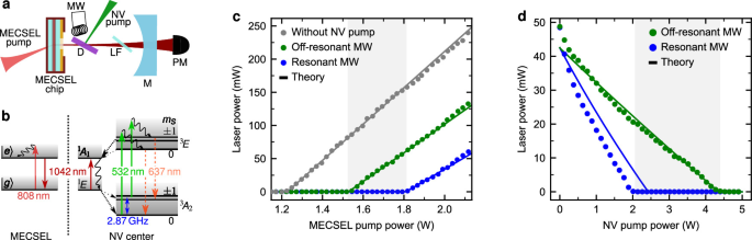
The two-media laser system used in this work is schematically shown in Fig. 1a. The optical gain medium is a membrane external cavity surface-emitting laser chip (MECSEL)50, which has a broad gain spectrum with a maximum at 1075 nm in an empty cavity. The gain chip was grown on a 4-inch GaAs substrate and consists of 11 InGaAs quantum wells. The membrane is sandwiched between two SiC heat spreaders with a thickness of 500 μm. One side of this stack has a highly-reflective coating for the MECSEL bandwidth and an anti-reflective coating for the pump wavelength at 808 nm and thus represents the first plane cavity mirror. The other side of the stack has an anti-reflective coating for the MECSEL bandwidth. Without any frequency filtering inside the cavity, the MECSEL runs multi-mode and exhibits a broad emission spectrum of approximately 6nm with the center at 1075 nm. The MECSEL gain spectrum is broad, making it possible to tune the wavelength down to 1042 nm with an intra-cavity birefringent filter (see below). The gain chip is optically pumped from the backside with a fiber-coupled diode laser at 808 nm (\({d}_{{\rm{core}}}=105\) μm, NA = 0.22), which we call MECSEL pump. The pump is collimated (Thorlabs F810SMA-780) and focused on the chip with a lens (f = 50 mm), resulting in a pump spot diameter of around 150 μm in the focus. The second cavity mirror (M) is concave (R = 95.1%, ROC = 100 mm) at a distance of Lcav ≈ 98.5 mm. This cavity geometry results in a cavity mode diameter of around 140 μm on the gain chip, leading to good mode overlap between the MECSEL pump and the cavity mode.
The diamond (D) is placed 28 mm away from the gain chip. Due to the cavity geometry, the cavity mode beam diameter at the diamond position is 280 μm. The diamond is oriented at Brewster’s angle, leading to reduced cavity losses for a p-polarized MECSEL mode. Two slightly different (100) oriented type 1b high-pressure-high-temperature (HPHT) diamond samples from the same batch were used in this work. Both diamonds have a geometry of (3 × 3) mm2 and a comparable thickness of ≈300 μm. The yellow starting material was commercially obtained from Element Six. The diamond used in Figs. 1 and 2 was pretreated with a low-pressure-high-temperature (LPHT) annealing at 1800 °C in a hydrogen atmosphere. This process leads to a decrease in the diamond absorption39,75. After this treatment, the diamond was electron irradiated with a fluence of 1 × 1018 cm−1 and an electron energy of 2 MeV. The diamond was then annealed for 2 h at 1000 °C to create nitrogen-vacancy (NV) centers. A high NV concentration of 2.05 ppm (93% NV−) was achieved, as was determined with the photoluminescence method from our previous work35. The diamond used in Fig. 3 was electron irradiated with a higher dose of 2 × 1018 cm−1, yielding a higher NV concentration of 3.77 ppm (92% NV−). Due to the much higher NV concentration, less NV pump power and microwave power are necessary to obtain a strong NV signal. Therefore, the linewidth, i.e., the intrinsic dynamic range, can be traded to achieve a better photon-shot-noise sensitivity limit, as demonstrated in Fig. 4. For both diamonds, the coherence times are comparable (\({T}_{2}^* \approx 200\,\,\text{ns}\)), as was determined in a confocal photoluminescence setup with a Ramsey sequence.
The NV centers are optically pumped with a 532 nm laser, which we call the NV pump. It is focused on the diamond with a lens (f = 125 mm) and adjusted to achieve good mode-matching with the cavity mode. The NV pump optically excites the NV centers from the triplet ground state 3A2 to the excited state 3E (see green arrow in Fig. 1b). From there, two relaxation paths back to the ground state exist. On the one hand, the NV center can fall back to the ground state under emission of a photon in the wavelength range from 637nm up to 850nm (orange dashed arrows)14. On the other hand, the NV center can undergo intersystem crossing (ISC, dashed black arrows) to the excited singlet state 1A1, followed by the singlet transition to the long-lived 1E and back to the ground state via ISC. The singlet transition (dark red arrow) exhibits a zero phonon line (ZPL) of 1042 nm, and phonon broadening seems to lead to a broadband absorption feature of the lower singlet state 1E47,48,49 despite very weak phonon sideband emission compared to the singlet ZPL emission76. The singlet transition is far less radiative than the triplet transition due to increased phonon transitions. Furthermore, the ISC is more probable for the mS = ±1 states (thickness of dashed arrows), making it possible to initialize to mS = 0 and to readout the spin state via a change in fluorescence after or during optical excitation14. Alternatively, the spin state can be determined via a change in absorption of a probe beam at 1042 nm45,46,71,77,78,79. The absorption is increased for the mS = ±1 states due to a favorable ISC and thus a higher population of the absorbing lower singlet state 1E. The spin-dependence of spontaneous emission and of absorption at 1042 nm is strongly enhanced by the long lifetime of the metastable lower singlet state 1E (>200 ns77).
A microwave field (MW) around 2.87 GHz is used to coherently drive the transition between mS = 0 and mS = ±1 in the triplet ground state 3A2 (blue arrow in Fig. 1b). Due to the Zeeman effect, the resonance frequencies of these spin transitions depend on the external magnetic field14. The microwave setup is the same as in previous work42,47.
A Lyot filter (LF) with a thickness of 3mm is used to tune the wavelength of the MECSEL down to the zero phonon line (ZPL) of the singlet transition at 1042 nm. The filter is made of crystal quartz, which is birefringent, leading to a wavelength-dependent phase difference δλ between the ordinary and extraordinary beam80,81,82. Only when the phase difference satisfies δλ = 2π does the Lyot filter preserve the polarization of the incident light, thereby minimizing cavity losses. By placing the filter at Brewster’s angle, only p-polarized modes will be allowed for the MECSEL due to decreased cavity losses. By rotating the optical axis of the Lyot filter, the refractive index for the ordinary and extraordinary, and thus the phase difference δλ, are changed, leading to a change in the MECSEL wavelength.
The MECSEL signal is measured in transmission with a power meter (PM). A 1000nm longpass filter is used to block the light from the two pump lasers. The transmitted cavity signal is also fiber-coupled to a grating spectrometer to resolve the spectrum of the two-media laser system. Usually, there is mode competition between different MECSEL modes with a distinct spectral distance of 0.4 nm due to the intra-cavity etalon introduced by the 500 μm thick SiC heat spreaders. We can monitor these modes in the spectrometer, and the laser system can be adjusted such that only one of those heat spreader modes turns on. This adjustment is strongly dependent on the operation point of the laser system, e.g., on the MECSEL pump power and the intra-cavity field. This leads to multi-mode operation, when the system is operated far from the threshold, as can be seen in deviations from the linear laser behavior in Fig. 1c, d.
Theoretical model
The theoretical model to describe the two-media laser system analytically is based on methods previously used27,34,42. In the following, the analytical model is described, and afterwards, the adaptation of the parameters to match the experimental data from the main text is discussed.
The model is based on finding an analytical steady-state solution to the equations of motion (EOMs) for both systems: the NV centers in diamond and the MECSEL. The two systems are coupled via the total number of photons inside the cavity. The relevant energy states and the nomenclature for the description are depicted in Fig. 5. By comparing this schematic with the level structure in Fig. 1b, one can assign the energy states and the optical transitions, which are relevant for the model. For simplicity, the MECSEL is assumed to be a two-level emitter. The strength of the NV and the MECSEL pump is given by the pumping rate ΛNV and Λge, respectively. The Li are the transition rates between different energy states. The NV ground state spin states are modeled coherently, i.e., with on- and off-diagonal density matrix elements, while all other transitions are modeled as rate equations. The coherent microwave coupling between mS = 0 and mS = ±1, i.e., the coupling between \(\left\vert 1\right\rangle\) and \(\left\vert 3\right\rangle\), is described as a Rabi oscillation with Rabi frequency Ω, detuning to the resonance Δ and dephasing \({{{\Gamma }}}_{{{\rm{13}}}}=1/{T}_{2}^{*}\). The coupling of the NV centers and the MECSEL to the cavity field is given by the cavity coupling strengths GS and Geg, respectively. Due to the short (long) lifetime of the upper (lower) singlet state \(\left\vert 5\right\rangle\) (\(\left\vert 6\right\rangle\))78 and the non-radiative decay pathway in the singlet transition, the NV center’s cavity effect is strongly dominated by absorption, and stimulated emission is negligible. Taking the contribution of stimulated emission into account led to the same results while having more complex analytical expressions. Thus, the NV center’s cavity coupling GS is modeled as a purely absorptive coupling. The strength of the cavity field is described by the number N of cavity photons.
Fig. 5: Energy levels and relevant transitions for the rate model describing the two-media laser system.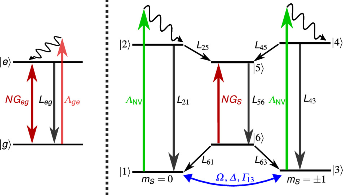
The NV center is modeled as a six-state system in combination with an optical excitation (green, ΛNV), spontaneous emission (black, L21 = L43) and a coherent microwave drive (blue, Ω, Δ, Γ13). The MECSEL is modeled as a two-level system, which is optically pumped (red, Λge), has a loss rate (black, Leg) and a gain to the cavity field (dark red, Geg). The NV center absorbs photons of the cavity field N with an absorption strength GS (dark red), leading to a coupling of the spin dynamics of the NV center and the cavity field.
Following the described nomenclature and the same procedure as in refs. 27,34,42, where the density matrix elements ρ11, ρ22, …ρ66, ρgg, ρee are populations of the corresponding states \(\left\vert \;j\right\rangle\) and the off-diagonal density matrix elements ρ13, ρ31 are the coherences of the corresponding states \(\left\vert 1\right\rangle\) and \(\left\vert 3\right\rangle\), the EOMs of the two systems are given by the following master equation
$${\dot{\rho }}_{13}=({{\rm{i}}}\Delta -{{{\Gamma }}}_{13}-{{{\Lambda }}}_{{{\rm{NV}}}}){\rho }_{13}+{{\rm{i}}}{{\Omega }}({\rho }_{11}-{\rho }_{33}),$$
(3)
$${\dot{\rho }}_{31}=-({{\rm{i}}}\Delta+{{{\Gamma }}}_{13}+{{{\Lambda }}}_{{{\rm{NV}}}}){\rho }_{31}+{{\rm{i}}}{{\Omega }}({\rho }_{33}-{\rho }_{11}),$$
(4)
$${\dot{\rho }}_{11}={{\rm{i}}}{{\Omega }}({\rho }_{13}-{\rho }_{31})-{{{\Lambda }}}_{{{\rm{NV}}}}{\rho }_{11}+{L}_{21}{\rho }_{22}+{L}_{61}{\rho }_{66},$$
(5)
$${\dot{\rho }}_{22}={{{\Lambda }}}_{{{\rm{NV}}}}{\rho }_{11}-({L}_{21}+{L}_{25}){\rho }_{22},$$
(6)
$${\dot{\rho }}_{33}={{\rm{i}}}{{\Omega }}({\rho }_{31}-{\rho }_{13})-{{{\Lambda }}}_{{{\rm{NV}}}}{\rho }_{33}+{L}_{43}{\rho }_{44}+{L}_{63}{\rho }_{66},$$
(7)
$${\dot{\rho }}_{44}={{{\Lambda }}}_{{{\rm{NV}}}}{\rho }_{33}-({L}_{43}+{L}_{45}){\rho }_{44},$$
(8)
$${\dot{\rho }}_{55}={L}_{25}{\rho }_{22}+{L}_{45}{\rho }_{44}-{L}_{56}{\rho }_{55}+{G}_{S}{\rho }_{66}N/{N}_{{{\rm{NV}}}},$$
(9)
$${\dot{\rho }}_{66}={L}_{56}{\rho }_{55}-{G}_{S}{\rho }_{66}N/{N}_{{{\rm{NV}}}}-({L}_{61}+{L}_{63}){\rho }_{66},$$
(10)
$${\dot{\rho }}_{gg}=-({{{\Lambda }}}_{ge}+{G}_{eg}N/{N}_{{{\rm{2M}}}}){\rho }_{gg}+({L}_{eg}+{G}_{eg}N/{N}_{{{\rm{2M}}}}){\rho }_{ee},$$
(11)
$${\dot{\rho }}_{ee}=({{{\Lambda }}}_{ge}+{G}_{eg}N/{N}_{{{\rm{2M}}}}){\rho }_{gg}-({L}_{eg}+{G}_{eg}N/{N}_{{{\rm{2M}}}}){\rho }_{ee}.$$
(12)
Here, the contribution from the MECSEL and the NV centers is taken into account by normalizing the number of cavity photons N to the number of MECSEL emitters N2M and NV centers NNV, respectively. For simplicity, the two quantities are assumed to be equal, and the strength of the contribution from both media is tuned via changing the pumping rates Λge, ΛNV and cavity couplings Geg, GS. The NV pumping rate is connected to the absorption cross section σ532 at 532 nm via ΛNV = σ532INV/Eph, where INV is the pump intensity, and Eph is the photon energy. The MECSEL pumping rate is chosen two orders of magnitude larger. The two systems are coupled via the EOM for the time-dependent number of cavity photons N, taken the total loss rate of the cavity κ into account:
$$\dot{N}=-{G}_{S}N{\rho }_{66}+{G}_{eg}N({\rho }_{ee}-{\rho }_{gg})-\kappa N.$$
(13)
To solve the system, the same procedure as in refs 27,34,42 is applied: We solve only for the steady-state solution \(\dot{\rho }=0,\dot{N}=0\). In the steady-state solution, all variables are time-independent constants and thus Eq. (3–12) can be solved independently, treating N as an unknown but constant parameter. We write the set of equations for both systems in (superoperator) matrix formalism. Then we solve for the kernel/nullspace of the matrix to get a solution for the density matrix elements dependent on all parameters, including the unknown N. Then, these solutions are inserted in Eq. (13) and the steady-state solution (\(\dot{N}=0\)) is solved. We obtain an analytical solution using Mathematica. The parameters that we used are literature values or are determined from our experimental setup and are summarized in Table 1.
Table 1 Parameters used for the modeling
The concentration of NV centers was measured via a calibrated photoluminescence brightness measurement with the procedure described in ref. 35 and then multiplied by the overlap of the cavity mode volume with the diamond plate to obtain the number of NV centers, NNV, contributing to the signal. The spin state decoherence rate \({{{\Gamma }}}_{13}=1/{T}_{2}^{*}\) was determined by measuring the \({T}_{2}^{*}\) coherence time in a confocal photoluminescence setup with a Ramsey sequence. The cavity loss rate κ was estimated by measuring the slope efficiency of the laser system for varying reflectivity of the cavity mirror as described in refs. 50,83.
To test whether our theoretical model can describe the experiment, the data from Fig. 1c are fitted with the analytical expression. We obtain the expression by taking the analytical solution for the number of cavity photons N, interpreting it as a function of the MECSEL pump rate Λge and then converting to laser powers with Pout = Ephκmirror N(Λge). Here, Eph is the photon energy, κmirror = 75 MHz is the cavity loss rate due to the outcoupling mirror, and N(Λge) is the photon number as a function of the MECSEL pump rate. The MECSEL pump power is PMP ∝ Λge with the assumed proportionality factor given in Table 1. We then adapt the following parameters to obtain a good match between our model and the experimental curves by fitting the given analytical expression to the data. To accurately describe the behavior around the threshold, only the first 10 data points above the threshold were used for this adaptation. First, the gray data in Fig. 1c is fitted to obtain the two-level emitter’s (MECSEL) spontaneous emission rate Leg and the cavity coupling Geg. The results are given in Table 2. With this, we have obtained the MECSEL parameters, which we later use to reproduce the other two curves in the same figure.
Table 2 Parameters obtained when adapting the analytical expressions to the experimental data in Fig. 1c
An alternative, simpler way to fit the MECSEL parameters confirms the same result: Without optically pumping the NV centers, the first term in Eq. (13) can be neglected since the populations are ρ55 = ρ66 = 0. When assuming detailed balance for the two-level system of the MECSEL, the steady-state solution for Eq. (13) is given as
$$N=\dfrac{({G}_{eg}-\kappa ){N}_{{{\rm{2M}}}}}{2\kappa {G}_{eg}}{{{\Lambda }}}_{ge}-\dfrac{({G}_{eg}+\kappa ){N}_{{{\rm{2M}}}}}{2\kappa {G}_{eg}}{L}_{eg}.$$
(14)
This describes a linear curve of the cavity photons N with respect to the pumping rate Λge. Fitting this comparably easy expression to the gray data from Fig. 1c leads to the same parameters for the MECSEL (see Table 2). This validates that the complex analytical expression obtained by the procedure explained above describes the case without optical pumping accurately.
To test the model in regard to the contribution of the NV centers, the green data from Fig. 1c, where the green NV pump laser is turned on, is fitted with the analytical expression. The MECSEL parameters determined by the previous fitting are inserted, and the detuning is chosen to be far away from the resonance (Δ = 0.87 GHz, as was used in the experiments). Thus, the only free parameter for the fitting is GS, which describes the strength of cavity field absorption by the NV centers, i.e., the coupling of the NV centers to the cavity field. The obtained value for GS, which makes the analytical solution fit the obtained data best, is given in Table 2. We point out that by turning on the green NV pump laser (and thus the NV absorption), two parameters in the plot are changed: the laser threshold and the slope of the curve, i.e., the slope efficiency of the laser. With the variation of a single model parameter, GS, to a complicated analytical solution, we were able to reproduce both parameter changes, indicating that the model is a good description of the physics in the experimental data.
Next, we regard the blue curve in Fig. 1c, where additionally the microwave drive is turned resonant and thus Rabi driving mixes the ground state spin states. We use again one free parameter in the analytical solution: the Rabi driving strength Ω, to now reproduce the blue data with our model. The MECSEL parameters and the strength of the NV absorption obtained before are inserted in the model. The obtained value for Ω, which makes the analytical solution fit the obtained data best, is given in Table 2. Again, two experimental parameter changes (threshold and slope) are reproduced by adapting one model parameter.
The fitting for the data in Fig. 1d was performed slightly differently. The green curve is matched to the data by adapting the MECSEL parameters (Leg = 5.1 MHz, Geg = 354 MHz). We note here that these adaptations are justified due to slightly different experimental conditions, like cavity adjustments, NV pump overlap and antenna positioning compared to Fig. 1c. The blue curve was obtained from the same MECSEL parameters as the green curve and by inserting the values for GS and Ω from Table 2. The resulting threshold shift (without adapting any parameter) reproduces the experimental threshold shift within reasonable bounds.
Photon-shot-noise sensitivity limit
The continuous wave (cw) sensitivity \({\eta }_{B}={\sigma }_{B}\sqrt{T}\) is a measure of the precision of a magnetometer which is independent of the measurement time T. The standard deviation of a magnetic field σB can be rewritten using error propagation as σB = ∣∂B/∂I∣σI. Here, I is the photon rate in the signal of optically detected magnetic resonance (ODMR) experiments. The standard deviation σI in the shot noise regime can be rewritten using Poissonian statistics as \({\sigma }_{I}=\sqrt{I}/\sqrt{T}\)56. This leads to the general definition of the photon-shot-noise (PSN) sensitivity limit as given by
$${\eta }_{B}(\nu )=\left| \dfrac{\partial B}{\partial \nu }\dfrac{\partial \nu }{\partial I}\right| {\sigma }_{I}\sqrt{T}=\dfrac{h}{{g}_{{{\rm{e}}}}{\mu }_{{{\rm{B}}}}}{\left| \dfrac{\partial I}{\partial \nu }\right| }^{-1}\sqrt{I(\nu )}.$$
(15)
Here h, ge, μB are the Planck constant, electron g-factor and Bohr magneton, respectively. The ODMR curve of the photon rate as a function of the microwave frequency is normally Lorentzian-shaped,
$$I(\nu )={I}_{0}\left(1-\dfrac{C\Delta {\nu }^{2}}{\Delta {\nu }^{2}+4{\nu }^{2}}\right),$$
(16)
where ν is the frequency shift from the resonance, Δν is the linewidth (full width at half maximum, FWHM), C is the contrast and I0 is the baseline of the Lorentzian56. The photon rate is connected to the detected power P and the energy per photon Eph via I(ν) = P(ν)/Eph. At this point, usually the assumption is made that the operating point of the best sensitivity in the ODMR curve ηB = ηB(νip) is achieved at the point of maximal slope in the Lorentzian curve, i.e., the inflection point \({\nu }_{{{\rm{ip}}}}=\Delta \nu /(2\sqrt{3})\) and that the signal strength at this point can be approximated by the baseline power I0 of the ODMR curve. These assumptions are valid only for small contrast and lead to the expression
$${\eta }_{B}\approx \dfrac{4}{3\sqrt{3}}\dfrac{h}{{g}_{{{\rm{e}}}}{\mu }_{{{\rm{B}}}}}\dfrac{\Delta \nu }{C\sqrt{{I}_{0}}}$$
(17)
for the PSN sensitivity limit of a cw magnetometer56. From this formula, it is often assumed that the PSN sensitivity limit scales linearly with enhanced contrast; however, this is only valid in the small contrast regime. In laser threshold magnetometry (LTM), where strong contrasts are achieved, this formula is not valid. The signal strength at the inflection point is I(νip) = I0(1 − 3C/4). Thus, the assumption I(νip) ≈ I0 is only valid for small contrast. Furthermore, the point of optimal sensitivity is shifted for larger contrast from the inflection point closer to the minimum of the ODMR curve. The fully correct formula for the PSN sensitivity limit without the small contrast approximation is determined by not fixing the operating point to the inflection point and not fixing the signal to the baseline signal. The formula is derived in detail in ref. 42 and can be given as a correction factor to the approximated formula
$${\eta }_{B}=\dfrac{4}{3\sqrt{3}}\dfrac{h}{{g}_{{{\rm{e}}}}{\mu }_{{{\rm{B}}}}}\dfrac{\Delta \nu }{C\sqrt{{I}_{0}}}\,\,\dfrac{\sqrt{{(3+{S}_{C}^{2})}^{3}(3+{S}_{C}^{2}-3C)}}{16{S}_{C}},$$
(18)
where SC describes the contrast-dependent shift of the optimal operating point (oop)42,
$${\nu }_{{{\rm{oop}}}}={\nu }_{{{\rm{ip}}}}{S}_{C}={\nu }_{{{\rm{ip}}}}\sqrt{C-1+\sqrt{{C}^{2}-5C+4}}.$$
(19)
Approaching unitary contrast shifts the operating point from the inflection point to the minimum of the ODMR resonance. The general equation for the PSN sensitivity limit scales super-linearly with the ODMR contrast, leading to an even stronger improvement when approaching unitary contrast. For a contrast of C=99.99%, the correction factor between the general Eq. (18) and the approximated Eq. (17) is approximately three, while additionally having the typical linear improvement of the PSN sensitivity limit with contrast.
The new Eq. (18) for the PSN sensitivity limit is experimentally verified by analyzing the red ODMR measurement from Fig. 2a. The results are given in Fig. 3a. The red curve was determined using Eq. (15) with I(ν) being the Lorentzian fit of the measurement data. The dotted line represents the results for the PSN sensitivity limit determined via the fit parameters of the Lorentzian using the typically assumed Eq. (17). The dashed line marks the PSN sensitivity limit determined by using the same fit parameters but the new and general valid Eq. (18) from42. There is a good overlap between the results for the general definition of the PSN sensitivity limit (see Eq. (15)) and the new Eq. (18) from42. This clearly demonstrates that the commonly used Eq. (17) is only valid in the regime of small ODMR contrasts and can thus not be used to estimate the PSN sensitivity limit for LTM. This result marks the first experimental demonstration of a super-linear improvement of the PSN sensitivity limit with contrast. Additionally, as expected from the results in ref. 42, the point of optimal PSN sensitivity shifts from the point of inflection for small contrasts to the minimum of the ODMR curve for higher contrasts. This shift can also be seen in the difference between the determination methods of the PSN sensitivity limit via the fit parameters (dashed and dotted line in Fig. 2d). The slightly worse sensitivity when approaching exactly the ODMR resonance is due to a contrast just below 100% (see Fig. 2a). When the hyperfine interaction of the NV centers with the 14N atom is visible in the ODMR spectrum and the hyperfine lines are not clearly separated, the fit function needs to be modified to a sum of three Lorentzian functions, as shown in Fig. 3b. When clearly separating the hyperfine line, e.g. by polarization of one state or by further decreasing the linewidth, Eq. (18) can be used to determine the PSN sensitivity limit. When the resonances are overlapping, as in Fig. 3b, Eq. (18) is not directly applicable, and Eq. (15) needs to be used to determine the PSN sensitivity limit (see Fig. 3c). Nevertheless, the super-linear improvement of the PSN sensitivity limit with contrast is still valid.