
1. Introduction
Direct numerical simulations (DNS) that resolve turbulent flows down to the Kolmogorov scales remain reserved for very few academic test cases. For simulations of wall-bounded turbulence, even stricter resolution requirements can apply because of the potentially very thin boundary layer. Alternatively, large eddy simulations (LES) can be performed, that solve for the spatially filtered flow field (Sagaut Reference Sagaut2005). In wall-resolved LES (WRLES) the filter width approaches zero close to the wall, which minimises the modelling required in the near-wall region, but only enables moderate coarsening of the mesh compared with DNS (Bose & Park Reference Bose and Park2018). The only computationally feasible alternative for most of the applications are wall-modelled LES (WMLES) that maintain a coarse mesh resolution throughout the computational domain, but that require specific modelling close to the wall to account for the subfilter effects in the turbulent boundary layer.
Despite WMLES being widely used for decades, the modelling interventions close to the wall remain mainly empirical and often rely on modelling assumptions that are difficult to justify. The commonly used wall-shear stress models assume a mean velocity profile for the instantaneous filtered velocity close to the wall in order to estimate the wall-shear stress of the unfiltered velocity. This estimated wall-shear stress is used to derive a Neumann boundary condition for the filtered flow field. However, since the velocity and the filtered velocity are different quantities that are governed by different equations, it is inconsistent to assume that the filtered velocity possesses the same wall-shear stress as the unfiltered velocity. Furthermore, the wall-shear stress is not directly available in the LES framework, where only filtered quantities are known, which is why the wall-shear stress is typically estimated by assuming a mean velocity profile (Deardorff Reference Deardorff1970; Schumann Reference Schumann1975) or by solving a transport equation for the mean velocity profile (Balaras, Benocci & Piomelli Reference Balaras, Benocci and Piomelli1996; Cabot & Moin Reference Cabot and Moin2000). Strictly speaking, these mean velocity profiles and solutions of the transport equations do not correspond to the instantaneous filtered velocity that is solved for in an LES.
An alternative wall-modelling approach to the wall-shear stress modelling is to assume a spatially varying filter with a filter width that approaches zero near the wall. A spatially varying filter width leads to additional terms that appear in the filtered equations for the fluid, and, at least with an elliptic differential filter, causes a non-zero velocity at the wall, even though the filter width is zero. In the dynamic slip wall model proposed by Bose & Moin (Reference Bose and Moin2014), one remaining parameter controlling the spatial change of the filter width is computed with a dynamic procedure. An important advantage of the dynamic slip wall model is that no assumptions on the underlying flow are required. However, the dynamic slip wall model is associated with some practical difficulties. It may be argued that a filter width that approaches zero close to the wall also requires a significantly refined mesh near the wall, which would lead to a computational cost of the order of WRLES, and undermines the computational advantage of WMLES. Another difficulty of the dynamic slip wall model is that the filter is non-uniform and, therefore, spatial derivatives and filtering do not commute, resulting in one additional closure term for each spatial derivative in the governing flow equations (Moser, Haering & Yalla Reference Moser, Haering and Yalla2021). There is a general consensus that these commutation errors can have a significant impact (Ghosal & Moin Reference Ghosal and Moin1995; Van Der Bos & Geurts Reference Van Der Bos and Geurts2005; Yalla et al. Reference Yalla, Oliver, Haering, Engquist and Moser2021), which may also be the case in the dynamic slip wall model.
There is more than one possible approach to define the flow quantities in LES in the vicinity of a wall. However, for an accurate modelling framework, it is essential to consistently account for all the consequences of the definition of flow quantities close to the wall, which is not necessarily the case for existing approaches. In a recent study, a novel LES wall-modelling framework is proposed that applies the so-called volume filtering initially introduced by Anderson & Jackson (Reference Anderson and Jackson1967) and that consistently accounts for all closures that arise (Hausmann & van Wachem Reference Hausmann and van Wachem2025b
).
In the present paper, we rigorously derive a formally exact expression for the slip and penetration boundary condition that arises when volume filtering a wall-bounded flow. This expression depends only on known filtered quantities. The resulting wall-modelling strategy does not make any a priori assumptions on the flow field and does not contain any free parameters, except for the filter width. After introducing the filtering framework in § 2, the wall-boundary conditions are derived in § 3 and validated in § 4, before the paper is concluded in § 5.
2. Spatial filtering of wall-bounded flows
Volume filtering of a generic flow quantity

$\varPhi$
is defined as (Anderson & Jackson Reference Anderson and Jackson1967)
(2.1)
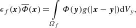
\begin{align} \epsilon _{{f}}(\boldsymbol{x}) \overline {\varPhi }(\boldsymbol{x}) = \int \limits _{\varOmega _{{f}}}\varPhi (\boldsymbol{y})g(|\boldsymbol{x}-\boldsymbol{y}|) \mathrm{d}V_y, \end{align}
where

$\varOmega _{{f}}$
is the domain occupied by fluid and

$g$
is a filter kernel that satisfies
(2.2)
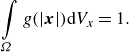
\begin{align} \int \limits _{\varOmega }g(|\boldsymbol{x}|) \mathrm{d}V_x = 1. \end{align}
Although the filter can, in principle, be any function that satisfies (2.2), in this work, the filter kernel is chosen to be a Gaussian with a standard deviation

$\sigma$
, which is referred to as filter width. In addition to the volume-filtered quantity,

$\overline {\varPhi }$
, volume filtering introduces an additional quantity, the fluid volume fraction,

$\epsilon _{{f}}$
, which is defined as
(2.3)
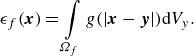
\begin{align} \epsilon _{{f}}(\boldsymbol{x}) = \int \limits _{\varOmega _{{f}}} g(|\boldsymbol{x}-\boldsymbol{y}|)\mathrm{d}V_y. \end{align}
The fluid volume fraction indicates which fraction of the volume in the filtered space is occupied by fluid at every point in space. In the limit of

$\sigma \rightarrow 0$
,

$\epsilon _{{f}}$
is either zero or one, but for finite filter widths,

$\epsilon _{{f}}$
can take any real value between zero and one.
The filter width can be chosen uniform in space, which avoids additional commutation closures in spatial derivatives, and, at a sufficient distance from the wall, the definition of volume filtering equals the definition of classical filtering in LES of unconfined flows.
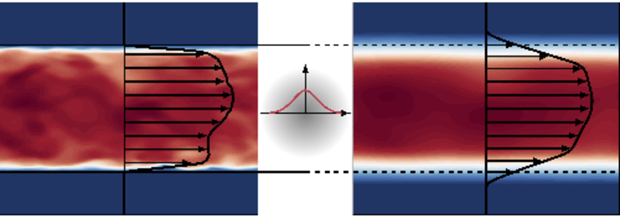
In figure 1, the effect of volume filtering on a wall-bounded flow is shown with the example of a flow between two flat plates. In the original unfiltered flow, the flow quantities are exclusively defined inside the flow domain and no-slip, no-penetration boundary conditions apply at the walls. Similarly to classical filtering in unconfined flows, volume filtering reduces the amplitudes of large wavenumbers. In addition, volume-filtered flow quantities are also defined outside the flow domain, but rapidly approach zero with increasing distance from the boundary of the flow domain. Consequently, the volume-filtered velocity at the location of the walls is not zero, but generally takes a finite value. Note that volume-filtered flow quantities that are non-zero outside the flow domain still describe a flow that is exclusively inside the flow domain, and that there is no dependency of the volume-filtered variables on unfiltered variables outside the flow domain. Volume filtering is a mathematical operation that projects the flow quantities defined inside a confined domain

$\varOmega _{{f}}$
onto an infinite domain

$\varOmega$
. Solving the flow in the volume-filtered space is numerically advantageous because a coarser resolution can be used. However, the flow physics remain the same whether they are solved in the unfiltered or volume-filtered space, given that the correct closure terms are applied to the volume-filtered equations.
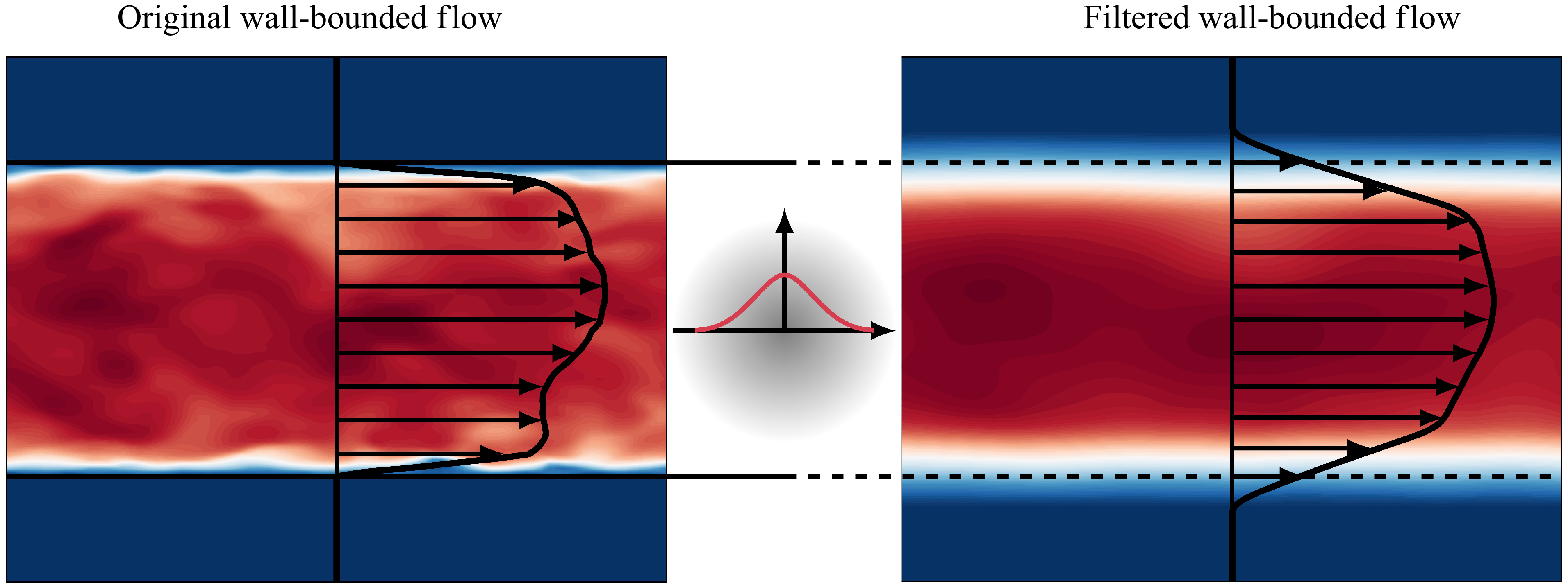
Figure 1. Visualisation of volume filtering with the example of a turbulent channel flow.
The equations governing the volume-filtered flow of a fluid with constant density,

$\rho _{{f}}$
, and constant dynamic viscosity,

$\mu _{{f}}$
, are obtained by applying the volume-filtering operation to the Navier–Stokes equations (Hausmann et al. Reference Hausmann, Chéron, Evrard and van Wachem2024a
)
(2.4)
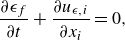
\begin{align} \dfrac {\partial \epsilon _{{f}}}{ \partial t} + \dfrac {\partial u_{\epsilon ,i}}{\partial x_i} &= 0, \end{align}
(2.5)

\begin{align} \rho _{{f}}\dfrac {\partial u_{\epsilon ,i}}{\partial t} + \rho _{{f}}\dfrac {\partial }{\partial x_j}(u_{\epsilon ,i}u_{\epsilon ,j}) &= -\dfrac {\partial p_{\epsilon }}{\partial x_i} +\mu _{{f}} \dfrac {\partial ^2u_{\epsilon ,i}}{\partial x_j \partial x_j} -s_i\color {black} + \mu _{{f}} \mathcal{E}_i- \rho _{{f}}\dfrac {\partial }{\partial x_j}\tau _{\textit{sfs},\textit{ij}}, \\[9pt] \nonumber \end{align}
where the volume-filtered velocity and pressure are denoted as

$u_{\epsilon ,i}=\epsilon _{{f}}\overline {u}_i$
and

$p_{\epsilon }=\epsilon _{{f}}\overline {p}$
. Three closure terms arise in the volume-filtered momentum equation,

$s_i$
,

$\mathcal{E}_i$
and

$\tau _{\textit{sfs},\textit{ij}}$
that are discussed in detail in Hausmann et al. (Reference Hausmann, Chéron, Evrard and van Wachem2024a
). The viscous closure,

$\mathcal{E}_i$
, can be shown to vanish in the case of stationary walls and the subfilter stress tensor,

$\tau _{\textit{sfs},\textit{ij}}$
, which is similar to the subfilter stress tensor in LES of unconfined flows, requires modelling.
The momentum source,

$s_i$
, arising from the presence of the walls is defined as
(2.6)
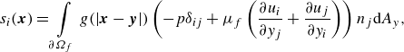
\begin{align} s_i(\boldsymbol{x}) = \int \limits _{\partial \varOmega _{{f}}}g(|\boldsymbol{x}-\boldsymbol{y}|)\left (-p \delta _{ij} + \mu _{{f}} \left (\dfrac {\partial u_i}{\partial y_j}+\dfrac {\partial u_j}{\partial y_i}\right )\right )n_j\mathrm{d}A_y, \end{align}
where

$\mathrm{d}A$
is the area of an infinitesimal wall element and

$n_j$
is the wall normal vector. The momentum source,

$s_i$
, contains the unfiltered pressure and the unfiltered viscous stresses and represents the local stresses exerted from the wall to the fluid. Due to the volume-filtering operation, these stresses are distributed over a region close to the wall, the size of which depends on the filter width. Accurate modelling of

$s_i$
is essential to predict the correct effect of the walls on the flow.
The modelling of

$s_i$
is a central aspect of the volume-filtered WMLES (VF-WMLES) introduced in Hausmann & van Wachem (Reference Hausmann and van Wachem2025b
) and Hausmann et al. (Reference Hausmann, Elmestikawy and van Wachem2024b
). The general idea is to discretise (2.6) by dividing the wall into small surface segments, each with an area

$\Delta A_l$
and a centre

$X_l$
, such that
(2.7)
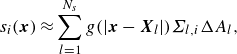
\begin{align} s_i(\boldsymbol{x}) \approx \sum _{l=1}^{N_{{s}}} g(|\boldsymbol{x}-\boldsymbol{X}_l|)\varSigma _{l,i} \Delta A_l, \end{align}
where

$\varSigma _{l,i}$
is the normal fluid stress vector at the wall segment

$l$
, which is assumed to be constant over the surface segment

$l$
. Since volume-filtered flow quantities are generally non-zero in the close vicinity of the wall outside the flow domain, the numerical domain for the solution must be chosen slightly larger than the flow domain.
In the recently proposed VF-WMLES, the normal fluid stress vector at each surface segment,

$\varSigma _{l,i}$
, is determined such that the correct volume-filtered velocity at the surface segment is obtained (Hausmann et al. Reference Hausmann, Elmestikawy and van Wachem2024b
; Hausmann & van Wachem Reference Hausmann and van Wachem2025b
). Therefore, the central aspect of the VF-WMLES that determines the accuracy of the predictions is how the volume-filtered velocity at the surface segment is obtained. In the following, we derive a formally exact expression for this volume-filtered velocity at the wall that depends only on volume-filtered quantities.
3. Derivation of the wall-boundary condition
For the derivation of the expression for the volume-filtered velocity at a point on the wall,

$u_{\epsilon ,i}|_{{w}}$
, we consider a coordinate system that has its origin at the arbitrarily shaped wall. There are two wall-tangential coordinate directions,

$x_s$
and

$x_t$
, and one wall-normal coordinate direction,

$x_n$
, pointing into the fluid.
We begin by deriving

$u_{\epsilon ,i}|_{{w}}$
by assuming that the unfiltered fluid velocity varies much more rapidly in the wall-normal direction than in the wall-tangential directions. Therefore, filtering near the wall is assumed to be predominantly a filtering in the wall-normal direction and the volume-filtered velocity at the wall is approximately given as
(3.1)
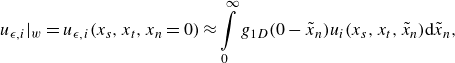
\begin{align} u_{\epsilon ,i}|_{{w}} = u_{\epsilon ,i}(x_{{s}},x_{{t}},x_{{n}}=0)\approx \int \limits _0^{\infty }g_{1{D}}(0-\tilde {x}_{{n}})u_i(x_{{s}},x_{{t}},\tilde {x}_{{n}}) \mathrm{d}\tilde {x}_{{n}}, \end{align}
where

$g_{1\textit{D}}$
is a one-dimensional Gaussian filter kernel. After deriving

$u_{\epsilon ,i}|_{{w}}$
for filtering in the wall-normal direction, we show later in this section how to extend the derivation considering filtering in all three directions.
The unfiltered fluid velocity at the wall is expanded as an infinite Taylor series expansion in the wall-normal direction, such that
(3.2)
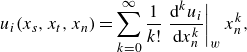
\begin{align} u_i(x_{{s}},x_{{t}},x_{{n}}) &= \sum _{k=0}^\infty \dfrac {1}{k!}\left .\dfrac {\mathrm{d}^ku_i}{\mathrm{d}x_{{n}}^k} \right |_{{w}} x_{{n}}^k, \end{align}
where

$\boldsymbol{\cdot }|_{{w}}$
indicates a quantity evaluated at the wall. Filtering of a monomial of order

$k$
in the wall-normal direction with a one-dimensional Gaussian is given as
(3.3)
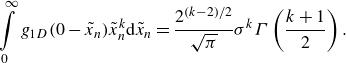
\begin{align} \int \limits _0^{\infty }g_{1{D}}(0-\tilde {x}_{{n}})\tilde {x}_{{n}}^k \mathrm{d}\tilde {x}_{{n}} = \dfrac {2^{(k-2)/2}}{\sqrt {\pi }}\sigma ^k \varGamma \left ( \dfrac {k+1}{2} \right ). \end{align}
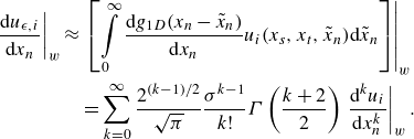
After inserting (3.2) into the definition of filtering given in (3.1) and replacing each filtered monomial with (3.3), the volume-filtered fluid velocity at the wall can be expressed as infinite series expansion
(3.4)
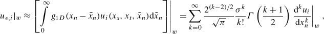
\begin{align} u_{\epsilon ,i}|_{{w}} &\approx \left .\left [\int \limits _0^{\infty }g_{1{D}}(x_{{n}}-\tilde {x}_{{n}})u_i(x_{{s}},x_{{t}},\tilde {x}_{{n}}) \mathrm{d}\tilde {x}_{{n}}\right ] \right |_{{w}} = \sum _{k=0}^\infty \dfrac {2^{(k-2)/2}}{\sqrt {\pi }}\dfrac {\sigma ^k}{k!} \varGamma \left ( \dfrac {k+1}{2} \right ) \left .\dfrac {\mathrm{d}^ku_i}{\mathrm{d}x_{{n}}^k} \right |_{{w}}, \end{align}
where

$\varGamma$
indicates the gamma function, i.e. a generalisation of the factorial function for complex numbers. Note that

$\boldsymbol{\cdot }|_{{w}}$
means that

$x_{{n}}=0$
, i.e. that a quantity is evaluated at the wall. This series expansion is not suitable for approximating

$u_{\epsilon ,i}|_{{w}}$
in a simulation because it contains the unfiltered velocity as an unknown. However, a similar expression can be obtained for the first derivative of the volume-filtered velocity in the wall-normal direction
(3.5)
\begin{align} \left . \dfrac {\mathrm{d} u_{\epsilon ,i}}{\mathrm{d}x_{{n}}}\right |_{{w}} &\approx \left .\left [ \int \limits _0^{\infty }\dfrac {\mathrm{d}g_{1{D}}(x_{{n}}-\tilde {x}_{{n}})}{\mathrm{d} x_{{n}}}u_i(x_{{s}},x_{{t}},\tilde {x}_{{n}}) \mathrm{d}\tilde {x}_{{n}}\right ] \right |_{{w}} \nonumber \\ & \quad = \sum _{k=0}^\infty \dfrac {2^{(k-1)/2}}{\sqrt {\pi }}\dfrac {\sigma ^{k-1}}{k!} \varGamma \left ( \dfrac {k+2}{2} \right ) \left .\dfrac {\mathrm{d}^ku_i}{\mathrm{d}x_{{n}}^k} \right |_{{w}}. \end{align}
Analogously, the

$l$
th derivative of the volume-filtered velocity in the wall-normal direction can be derived for

$l\gt 1$
to be given as
(3.6)
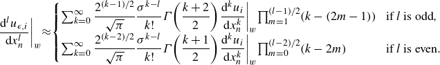
\begin{align} \left . \dfrac {\mathrm{d}^l u_{\epsilon ,i}}{\mathrm{d}x_{{n}}^l}\right |_{{w}} \! \approx \! \begin{cases} \sum _{k=0}^\infty \dfrac {2^{(k-1)/2}}{\sqrt {\pi }}\dfrac {\sigma ^{k-l}}{k!} \varGamma \!\left ( \dfrac {k+2}{2}\right )\! \left .\dfrac {\mathrm{d}^ku_i} {\mathrm{d}x_{{n}}^k} \right |_{{w}}\!\prod _{m=1}^{(l-1)/2} (k-(2m-1)) & \!\text{if }l\text{ is odd},\\ \sum _{k=0}^\infty \dfrac {2^{(k-2)/2}}{\sqrt {\pi }}\dfrac {\sigma ^{k-l}}{k!} \varGamma \! \left ( \dfrac {k+1}{2}\right )\! \left .\dfrac {\mathrm{d}^ku_i} {\mathrm{d}x_{{n}}^k} \right |_{{w}}\! \prod _{m=0}^{(l-2)/2} (k-2m) & \!\text{if }l\text{ is even} .\end{cases} \end{align}
This can be written as an equation system with an infinite number of variables and an infinite number of equations
(3.7)
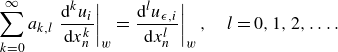
\begin{align} \sum _{k=0}^\infty a_{k,l}\left .\dfrac {\mathrm{d}^ku_i} {\mathrm{d}x_{{n}}^k} \right |_{{w}} = \left . \dfrac {\mathrm{d}^l u_{\epsilon ,i}}{\mathrm{d}x_{{n}}^l}\right |_{{w}}, \quad l=0,1,2,\ldots . \end{align}
Assuming that

$a_{k,l}$
is not singular, inverting the infinite matrix

$a_{k,l}$
gives an analytical expression for the unfiltered velocity and all of its derivatives in the wall-normal direction at the wall. The resulting expression depends only on volume-filtered quantities.
The magnitude of

$a_{k,l}$
decreases rapidly for large

$k$
, and the infinite sum in (3.7) can be truncated after

$k=N$
, which leads to a truncation error that is proportional to

$\sigma ^{N+1-l}$
. Since an expression for

$u_{\epsilon ,i}|_{{w}}$
is desired, that is,

$l=0$
, the error is proportional to

$\sigma ^{N+1}$
. The remaining truncated equation system contains

$N+1$
unknowns (the unfiltered Dirichlet boundary condition

$u_i|_{{w}}$
is known but

$u_{\epsilon ,i}|_{{w}}$
is unknown). Considering the derivatives of the volume-filtered velocity up to order

$l=N$
leads to

$N+1$
equations for the

$N+1$
unknowns. After solving the linear equation system, the volume-filtered velocity at the wall is given as
(3.8)
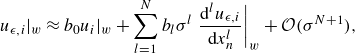
\begin{align} u_{\epsilon ,i}|_{{w}} \approx b_0u_i|_{{w}} + \sum _{l=1}^Nb_l \sigma ^l \left . \dfrac {\mathrm{d}^l u_{\epsilon ,i}}{\mathrm{d}x_{{n}}^l}\right |_{{w}} + \mathcal{O}(\sigma ^{N+1}), \end{align}
where the coefficients

$b_l$
are given in table 1 up to

$N=4$
. Equation (3.8) is referred to as formally exact because it can be formulated theoretically for any order of accuracy. However, in practice the series expansion is truncated and the boundary condition becomes an approximation. A script to derive (3.8) and the coefficients given in table 1 is openly available (Hausmann & van Wachem Reference Hausmann and van Wachem2025a
). Note that, if

$N=1$
, (3.8) is similar to the empirical expression that has been previously used for the boundary conditions in the scope of the VF-WMLES but with different coefficients

$b_0$
and

$b_1$
(Hausmann & van Wachem Reference Hausmann and van Wachem2025b
).
Table 1. Coefficients for the expression for the volume-filtered velocity at the wall given in (3.8) up to

$N=4$
assuming filtering exclusively in the wall-normal direction.
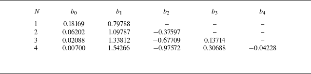
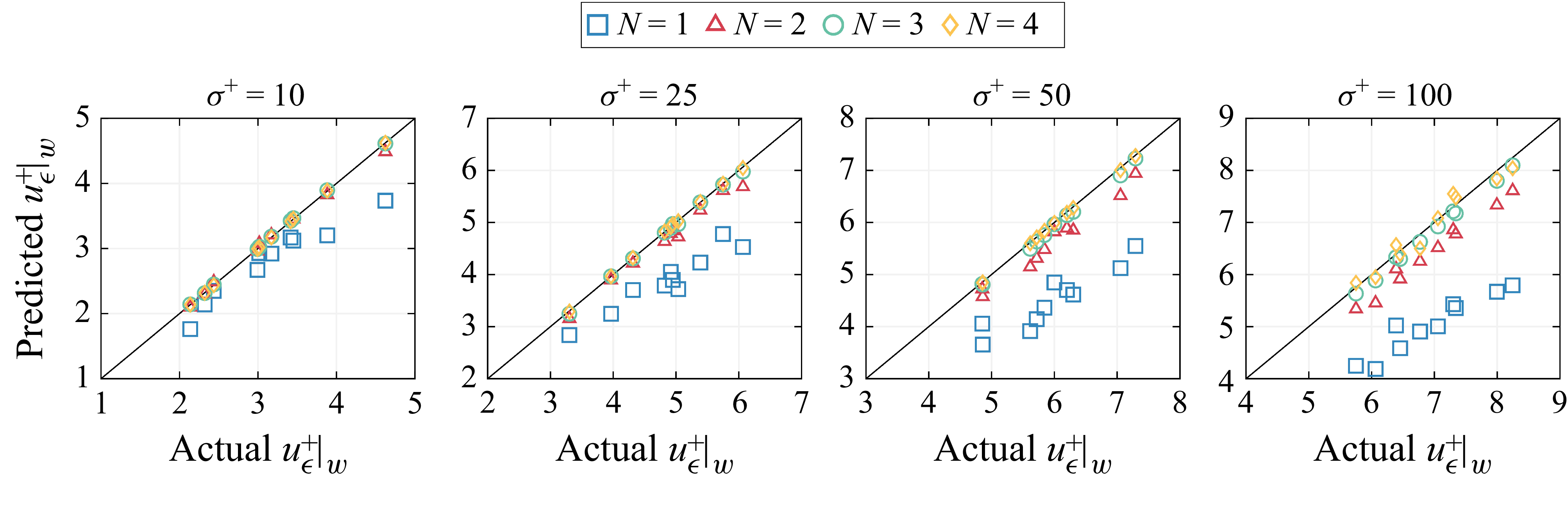
Figure 2. The volume-filtered streamwise velocity at the wall predicted by (3.8) up to order

$N$
for randomly chosen velocity profiles of a turbulent channel flow compared with the actual volume-filtered velocity at the wall obtained by explicit volume filtering of the velocity profiles for different filter widths.
In figure 2, the predicted volume-filtered velocity at the wall using (3.8) is compared with the explicitly volume-filtered instantaneous streamwise velocity profiles at randomly chosen positions in a turbulent channel flow for different

$N$
and different filter widths. The turbulent channel flow has a friction Reynolds number of

$\textit{Re}_\tau =1000$
and the instantaneous profiles are extracted from the Johns Hopkins turbulence database (Graham et al. Reference Graham2016). The streamwise direction is denoted as the

$x$
-direction. Note that the velocity profiles are only filtered in the wall-normal direction. Quantities with a superscript

$+$
are normalised with wall units. As can be seen from figure 2, the accuracy of the predicted volume-filtered velocity at the wall improves with increasing

$N$
. With increasing filter width, the truncation error increases. However, with

$N=2$
and

$\sigma ^+=100$
, which is a typical filter width used in WMLES, the error in predicting the volume-filtered velocity at the wall is small compared with other modelling errors that can be expected in such a coarse WMLES.
Although the right-hand side of (3.8) is exact up to an arbitrary order for filtering in the wall-normal direction, it is only an approximation for

$u_{\epsilon ,i}|_{{w}}$
because it neglects the filtering in the wall-tangential directions. However, it is straightforward to extend the derivation of the expression for the volume-filtered velocity at the wall to filtering in the wall-normal and wall-tangential directions, albeit algebraically more tedious. After expressing

$u_i$
as a three-dimensional Taylor series around the wall and replacing the one-dimensional-filtering operation given in (3.1) with the three-dimensional filtering as given in (2.1), the following expression for the volume-filtered velocity at the wall is obtained:
(3.9)
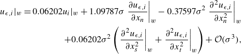
\begin{align} u_{\epsilon ,i}|_{{w}} = 0.06202 u_i|_{{w}} + 1.09787\sigma \left . \dfrac {\partial u_{\epsilon ,i}}{\partial x_{{n}}}\right |_{{w}}- 0.37597\sigma ^2 \left . \dfrac {\partial ^2 u_{\epsilon ,i}}{\partial x_{{n}}^2}\right |_{{w}} \nonumber \\+ 0.06202\sigma ^2 \left ( \left . \dfrac {\partial ^2 u_{\epsilon ,i}}{\partial x_{{s}}^2}\right |_{{w}} + \left . \dfrac {\partial ^2 u_{\epsilon ,i}}{\partial x_{{t}}^2}\right |_{{w}}\right ) + \mathcal{O}(\sigma ^{3}), \end{align}
which corresponds to

$N=2$
. This expression is exact up to terms proportional to

$\sigma ^{3}$
and higher-order expressions can be derived analogously. Note that the coefficients are different in the wall-normal and wall-tangential directions because the integration limits for convoluting the monomials with a Gaussian, as done in (3.3), are

$(-\infty ,\infty )$
for the wall-tangential directions instead of

$(0,\infty )$
for the wall-normal direction.
4.
A posteriori evaluation of the wall-boundary condition
The different orders of approximations of the volume-filtered velocity at the wall are compared in an a posteriori study of the turbulent flow over a periodic hill at

${\textit{Re}}_{H}=10595$
, where

${\textit{Re}}_{H}$
is the Reynolds number based on the height of the hill,

$H$
, and the bulk velocity at the crest of the hill,

$u_{{b}}$
. Periodic boundaries are employed in the streamwise (

$x$
) and the spanwise (

$z$
) directions and the flow domain is bounded by walls in the

$y$
direction. Further details of the flow configuration can be found in one of the many studies that exist in the literature on this exact flow configuration, which serves as a typical test case for LES wall models (see, e.g. Temmerman et al. Reference Temmerman, Leschziner, Mellen and Fröhlich2003; Fröhlich et al. Reference Fröhlich, Mellen, Rodi, Temmerman and Leschziner2005; Krank, Kronbichler & Wall Reference Krank, Kronbichler and Wall2018; Hausmann & van Wachem Reference Hausmann and van Wachem2025b
).
The flow simulations are performed with a finite volume solver with second-order spatial and temporal accuracy that is based on momentum weighted interpolation and a solution of the continuity and momentum equation in a single equation system (Denner & van Wachem Reference Denner and van Wachem2014; Bartholomew et al. Reference Bartholomew, Denner, Abdol-Azis, Marquis and van Wachem2018; Denner, Evrard & van Wachem Reference Denner, Evrard and van Wachem2020). A van Leer flux limiter is used and a dynamic time step is used to maintain a CFL number of

$0.1$
during the simulation. The flow is solved on a uniform mesh with a resolution of

$\Delta x = \Delta y = \Delta z = 0.07H$
, which means that there are between 28 and 43 mesh cells in the

$y$
direction between the channel walls, depending on the position in the channel. Based on the maximum wall-shear stress, the grid spacing in wall units corresponds to
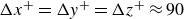
$\Delta x^+ = \Delta y^+ = \Delta z^+ \approx 90$
. Note that it is not required that the mesh is uniform and isotropic, but if the filter width is changing in space, additional closures appear that require modelling. The VF-WMLES are performed as briefly introduced in § 2 and explained in detail in Hausmann et al. (Reference Hausmann, Elmestikawy and van Wachem2024b
) and Hausmann & van Wachem (Reference Hausmann and van Wachem2025b
). The Vreman model is used as the subgrid-scale model (Vreman Reference Vreman2004).
In figure 3, the mean velocity profiles in the

$x$
and

$y$
directions obtained with the VF-WMLES are compared with the explicitly volume-filtered DNS velocity profiles of Krank et al. (Reference Krank, Kronbichler and Wall2018) filtered in the

$y$
direction. The volume-filtered velocity at the wall is obtained with (3.8) considering terms up to

$N=1$
(first-order), up to

$N=2$
(second-order) and

$N=2$
including the tangential direction as given in (3.9) (second-order tangential). The simulations are performed with three different filter widths

$\sigma /H=0.14$
,

$\sigma /H=0.105$
and

$\sigma /H=0.07$
, which correspond to

$\sigma /\Delta x =2$
,

$\sigma /\Delta x =1.5$
and

$\sigma /\Delta x =1$
, respectively. Note that, since the boundary conditions used in Hausmann & van Wachem (Reference Hausmann and van Wachem2025b
) are very similar to the first-order series expansion and lead to similar results, they are not added for comparison.
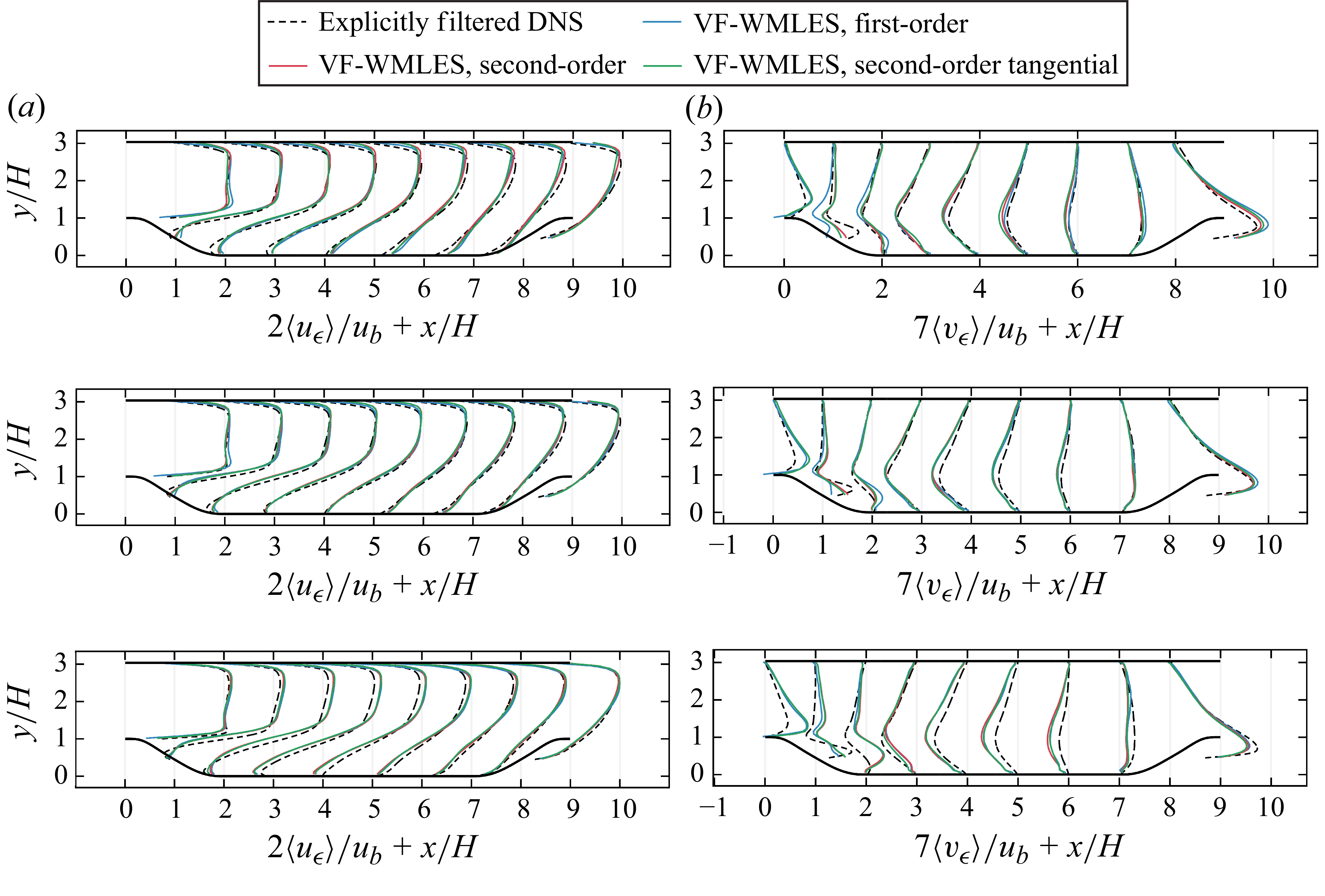
The streamwise mean velocity profiles are only weakly dependent on the boundary conditions for all of the three filter widths and most of the velocity profiles agree well with the explicitly volume-filtered DNS. More significant differences between the boundary conditions are observed for the mean velocity in the

$y$
direction, especially in the recirculation region

$0\leqslant x \leqslant 3H$
. In this region, the second-order boundary conditions generally lead to mean velocity profiles that are closer to the explicitly volume-filtered DNS than the first-order boundary condition, whereas including the wall-tangential variation of the velocity in the boundary conditions has no significant effect on the mean velocity profiles. The least accurate mean velocity profiles are obtained with the smallest filter width of

$\sigma /H=0.07$
. If the filter width is too small, the discretisation error can have a significant impact on the solution because the filtered flow field is not smooth enough to be sufficiently resolved by the mesh. If the discretisation error is larger than the modelling error, the results are expected to be only weakly dependent on the exact model for the boundary conditions used, which is the case for the mean volume-filtered velocity profiles obtained with

$\sigma /H=0.07$
. This suggests that a filter width of

$\sigma /H=0.07$
is too small for the present configuration.
To assess the accuracy of the VF-WMLES with the proposed boundary conditions in the context of the existing WMLES literature, the mean velocity profiles of the VF-WMLES with the first-order series expansion are compared with an equilibrium wall model. In figure 4, we compare the mean streamwise velocity profiles of the VF-WMLES with

$\sigma /H=0.105$
at

$x/H=2$
and

$x/H=6$
with the classical WMLES performed by Temmerman et al. (Reference Temmerman, Leschziner, Mellen and Fröhlich2003) using the Werner–Wengle (WW) wall-model together with the dynamic Smagorinsky (DSM) and the wall-adapted local eddy viscosity (WALE) subgrid-scale model. The simulations carried out by Temmerman et al. (Reference Temmerman, Leschziner, Mellen and Fröhlich2003) are performed on a curvilinear mesh with approximately 50 % more mesh cells than the present VF-WMLES and mesh refinement in critical regions, such as the crest of the hill. In addition to that, the mean velocity profiles obtained by Chang et al. (Reference Chang, Liao, Hsu, Liu and Lin2014) with an immersed boundary method (IBM) on a Cartesian mesh with the WW wall model and the DSM subgrid-scale model are shown. The simulations by Chang et al. (Reference Chang, Liao, Hsu, Liu and Lin2014) are carried out with a solver with second-order spatial accuracy and a mesh with more than four times as many mesh cells than in the present simulations. The mean velocity profiles predicted with the VF-WMLES and the classical WMLES using the WW wall model together with the WALE subgrid-scale model deviate only slightly from the explicitly volume-filtered DNS velocity profile. Combining the WW model with the DSM subgrid-scale model, however, leads to significant deviations for both, the simulations on the curvilinear mesh and the IBM simulations.
As seen from figure 4, the mean velocity profiles across the channel are not a direct measure of the accuracy of the wall-boundary conditions due to the significant influence of the subgrid-scale model. Therefore, the mean volume-filtered velocity at the wall is investigated, which is shown in figure 5 for the different boundary conditions and filter widths along the bottom wall. The DNS mean velocity profiles, which are only available at discrete

$x$
positions, are explicitly volume filtered in the wall-normal direction and are shown as a reference. As observed in figure 5, the wall-boundary condition obtained with the first-order series expansion predicts a too small volume-filtered velocity at the wall at the location of the crest of the hill (

$x=0$
and

$x=9H$
) for all of the three filter widths. With the second-order series expansions (with and without the tangential directions), the volume-filtered velocity at the crest of the hill is predicted accurately. In the recirculation region (

$0 \leqslant x \leqslant 3H$
), the volume-filtered velocity at the wall is negative, which is captured more accurately with the second-order series expansions than with the first-order series expansion. Including the tangential direction in the second-order series expansion has a negligible effect on the volume-filtered velocity at the wall, independent of the filter width.
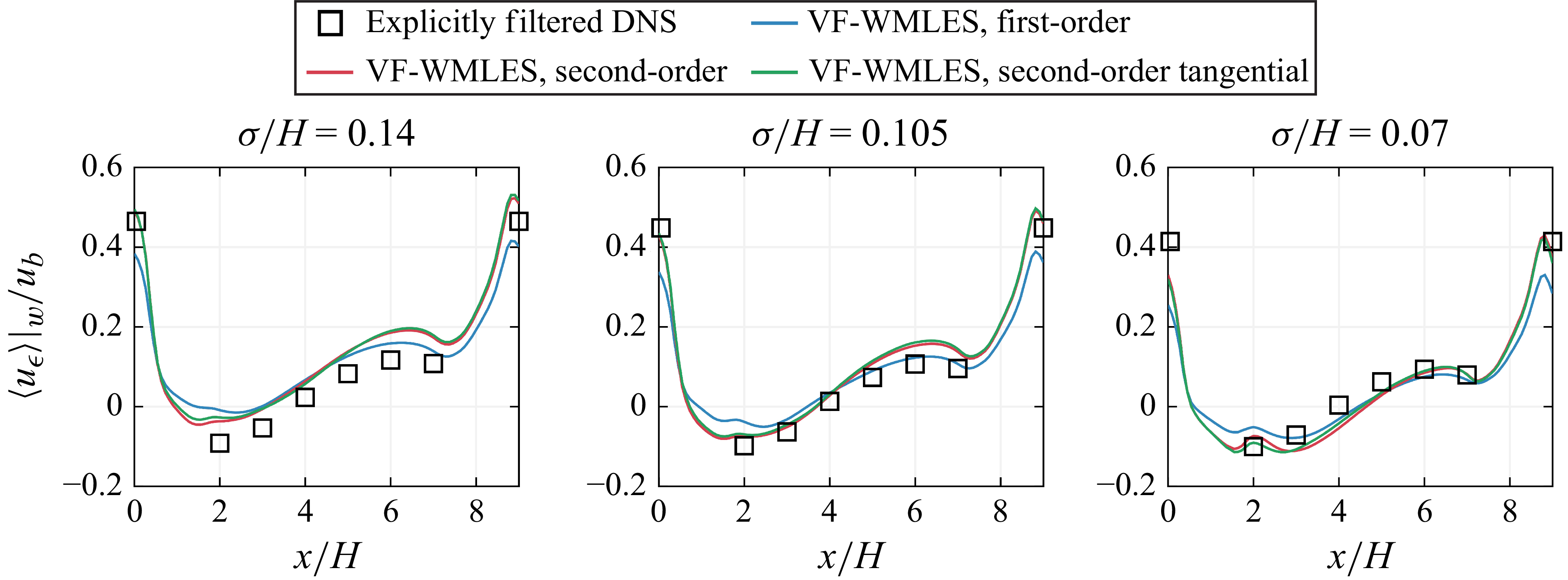
Figure 5. Volume-filtered velocity at the wall obtained with the VF-WMLES with different boundary conditions and filter widths compared with the volume-filtered velocity at the wall obtained by explicitly volume filtering the DNS velocity profiles.
With the intermediate filter width of

$\sigma /H=0.105$
, the best predictions of the volume-filtered velocity at the wall are achieved. For the small filter width, the discretisation error can have a significant contribution, and for the large filter width, there is an increased modelling error from the wall-boundary condition and from the subgrid-scale modelling. Therefore, the optimal filter width depends on the specific discretisation and the model for the subfilter stress tensor. Generally, the higher the spatial order of accuracy of the flow solver, the smaller the filter width can be chosen. However, the filter width should not be significantly smaller than

$\sigma /\Delta x =1$
to avoid excessive aliasing errors.
5. Conclusions
In the present paper, a formally exact expression for the filtered velocity at the boundaries of arbitrary flow domains is derived by rigorous application of the concept of volume filtering. This derivation does not make any a priori assumptions on the flow and is shown to lead to a suitable boundary condition for LES of wall-bounded flows. The derived expression is an infinite series expansion in powers of the filter width, and it depends only on quantities known in an LES. The contribution of each successive term in the series decreases as the order of the term increases. This means that the series can be truncated, and not all terms need to be retained. As shown in an a priori study with instantaneous velocity profiles of a turbulent channel flow, truncating the series expansion after terms proportional to the squared filter width leads to accurate predictions of the filtered velocity at the wall for filter widths typical for WMLES. In a posteriori studies using WMLES applied to turbulent flow over periodic hills, it is shown that the proposed boundary conditions can predict the mean velocity profiles and the filtered velocity at the boundary accurately. The proposed formally exact boundary conditions do not rely on any empirical parameters and are shown to be a promising alternative to classical WMLES with wall-shear stress models that make assumptions on the velocity profiles near the walls.