
Floquet Kitaev model
The Floquet Kitaev model is well understood because of a Majorana representation of the spins, which shows the free-fermion solvability of the model6,39. On each site, four Majorana operators {c, bx, by, bz} can be defined, such that the Pauli operations on the spin sites are
$${X}_{j}={\rm{i}}{c}_{j}{b}_{j}^{x},\quad {Y}_{j}={\rm{i}}{c}_{j}{b}_{j}^{y},\quad {Z}_{j}={\rm{i}}{c}_{j}{b}_{j}^{z},$$
(9)
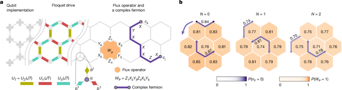
where \({c}_{j}^{2}=1\) and {cj, ck} = 0 for j ≠ k, and similarly for \({b}_{j}^{\alpha }\) (Extended Data Fig. 1a). This representation enlarges the Hilbert space, and the physical Hilbert space corresponds to the set of states |Ψ⟩ such that \({c}_{j}{b}_{j}^{x}{b}_{j}^{y}{b}_{j}^{z}| \psi \rangle =| \psi \rangle \) for all j. The model has a set of conserved quantities \({u}_{jk}={\rm{i}}{b}_{j}^{{\alpha }_{jk}}{b}_{k}^{{\alpha }_{jk}}\), where αjk is the Pauli operator associated with that bond. Note that these are conserved not just stroboscopically, but at all points throughout the drive. These can be thought of as a \({{\mathbb{Z}}}_{2}\) gauge field, and products of these operators around closed loops correspond to physical gauge-invariant conserved quantities, the fundamental instances of which are the flux operators shown in Extended Data Fig. 1a:
$${W}_{{\rm{P}}}=\prod _{\langle i,j\rangle \in {\hexagon}}{u}_{ij}.$$
(10)
These measure the flux through each of the plaquettes, and we refer to WP = +1 as flux-free. Each of the driving terms is then of the form
$$\exp \left\{-JT\frac{{\rm{\pi }}}{4}\sum _{\langle ij\rangle }{u}_{ij}{c}_{i}{c}_{j}\right\},$$
(11)
which is quadratic in the ci-Majorana fermion operators. These correspond to hopping operators for the c-fermions and perform a Majorana swap when JT = 1 (M-SWAP). This driving can be efficiently implemented on a quantum processor using C-PHASE gates and single-qubit rotations, as shown for the example of a single hexagonal plaquette in Extended Data Fig. 1b.
To monitor the dynamics of the emergent Majorana modes, we define measurable operators by pairing them with complex fermions. The paired fermion operators are then defined as fjk = (cj + iϕjkck)/2, where
$${\phi }_{jk}=\prod _{\langle l,m\rangle \in \text{path}\,(j,k)}{u}_{lm}$$
(12)
is a gauge string consisting of a product of the gauge fields along a path connecting the paired sites. This leads to a density operator
$${n}_{{\rm{F}}}(j,k)=\frac{1}{2}({\rm{i}}{\phi }_{jk}{c}_{j}{c}_{k}+1),$$
(13)
which can be written as a Pauli string. Under the Floquet dynamics, these paired fermions move around the system, as shown in Extended Data Fig. 1c.
Experimental procedures
CZ and C-PHASE gates are implemented by setting the qubit detuning close to the anharmonicity and harnessing a diabatic |11⟩ ⇄ |20⟩ swap to generate an arbitrary C-PHASE angle with minimal leakage51. Dominant errors come from CZ/C-PHASE entangling gates and final readout52 (Extended Data Fig. 2a). The Snake optimizer53,54 has been used to optimize qubits, coupler and readout parameters. A smaller contribution to the total error comes from the single-qubit microwave gates, which are calibrated using the Optimus calibration tools of Google55,56.
Dynamical decoupling
Idle qubits are exposed to errors over time. In particular, this is important for Hadamard tests such as the Floquet braiding experiment. In contrast to all other qubits, the ancilla is not part of the Floquet time evolution and is idle during this time. To quantify those errors under experimental conditions, we use the same circuit as in the actual Floquet braiding experiment but do not couple the ancilla to the system (Extended Data Fig. 2b). Therefore, the ancilla should remain in the |+⟩ state as no other operation is performed on it. In the Hadamard test, we would measure the expectation value of ⟨XA⟩ and ⟨YA⟩ and we, therefore, probe those two expectation values here. In Extended Data Fig. 2c, we would expect to measure +1 at all times for ⟨XA⟩ and 0 for ⟨YA⟩. However, we observe that ⟨XA⟩ decreases quickly, whereas ⟨YA⟩ increases at the same time. To mitigate this effect, we apply a simple form of dynamical decoupling57 by randomly applying X-X or Y-Y sequences on the idle ancilla. Extended Data Fig. 2d shows that this technique effectively reduces these errors rather well.
Randomized compiling
To address CZ-gate dependent errors, which can arise from imperfect gate calibration, we have applied randomized compiling to all CZ gates in all experiments. This technique58,59 involves inserting sets of Pauli operators before and after the CZ gates, leaving the total circuit invariant while significantly enhancing the overall performance. We repeated all experiments for 20 different twirling sets.
Noisy simulation
To further explore the effects of noise on our results, we perform noisy quantum trajectory simulations and compare them with experimental data (Extended Data Fig. 2e) of a two-plaquette setup, which is shown on the left-hand side. Because we use randomized compiling, we approximate CZ gate errors as a two-qubit depolarizing channel. In the simulation, we apply different error rates to each pair of qubits, obtained from two-qubit XEB experiments conducted just before the experimental data in Extended Data Fig. 2e was collected. We also include amplitude damping on the ancilla during the Floquet cycles to account for T1 decay, assuming a T1 of 25 μs. Finally, we include readout errors of 0.4% on the |0⟩ state and 2.5% on the |1⟩ state. This error model produces results that are qualitatively consistent with the experimental data: the overlap shows a decaying magnitude, r. Together with the results in Extended Data Fig. 2b–d, this agreement suggests the described error model with an additional coherent phase drift on the ancilla qubit (strongly mitigated by dynamical decoupling) reproduces our experimental observations.
Extended data and derivationsPreparation of initial states
To prepare a flux-free state, we use the circuit shown in Extended Data Fig. 3a for the seven-plaquette setup and the circuit shown in Extended Data Fig. 4 for the large system, which was introduced in refs. 16,42, where H is the Hadamard gate
$$H=\frac{1}{\sqrt{2}}\left[\begin{array}{cc}1 & 1\\ 1 & -1\end{array}\right]$$
and S denotes the phase gate given by
$$S=\left[\begin{array}{cc}1 & 0\\ 0 & i\end{array}\right].$$
After this initial preparation, fermions are paired vertically on z-bonds. In the main text, we denote this flux-free state as |ψFF⟩. For all experiments, we first prepare this flux-free state and then rearrange the fermions depending on the initial state needed. To preserve the fluxes, fermions can be rearranged by applying \({{\rm{e}}}^{-{\rm{i}}JT\frac{{\rm{\pi }}}{4}{({\alpha }_{jk})}_{j}{({\alpha }_{jk})}_{k}}\) with JT = 1 so that those operators correspond to swap operations of c-Majoranas of the respective bond (M-SWAP). Choosing the operator depending on the type of bond (x, y or z) preserves the flux. Extended Data Fig. 3b shows the step-by-step rearrangement of fermions for the initial state of Fig. 1b.
The circuit for the flux-free state preparation of the 58-qubit setup used in the e-m transmutation experiment, as well as the two layers of M-SWAP gates used for rearranging the fermions, is shown in Extended Data Fig. 4. For all other experiments, state preparation is detailed in the figures in the main text. Generally, we have chosen initial states to ensure that the circuits are as shallow as possible while yielding the clearest experimental results. For example, in the case of the spectral function, the only requirement for the initial state, apart from being flux-free, is that the protruding bond hosts a perfectly occupied fermion. Beyond that, the specific pairing of Majoranas in the rest of the system is irrelevant. As such, starting directly from the flux-free state yields the shallowest circuit. Notably, we have this freedom in the initial state, as we are probing properties of the Floquet operator rather than fine-tuned initial states.
Data analysis
For all datasets, we apply jackknife resampling before further analysis. The raw data for each experiment consists of 20 twirling sets, and each twirling set contains many measured data points. To estimate statistical uncertainties, we construct jackknife samples by systematically leaving out one entire twirling set at a time. More precisely, let θi denote the average for the ith twirling set. Then the ith jackknife sample ji is given by
$${j}_{i}=\frac{1}{{N}_{{\rm{twirling}}}-1}\mathop{\sum }\limits_{k\ne i}^{{N}_{{\rm{twirling}}}}{\theta }_{k}.$$
(14)
This procedure yields Ntwirling = 20 jackknife samples ji. When analysing a quantity f that depends on multiple measured variables, we construct jackknife samples for each variable on its own. Suppose our desired analysis function is a multivariate function f, then for each jackknife index i, we have a set of jackknife samples (ji, li, …) corresponding to all variables. Applying f to these jackknife samples yields 20 samples:
$${F}_{i}=f({j}_{i}\,,{l}_{i},\ldots ).$$
(15)
Finally, the jackknife mean and standard error are given by
$$\overline{F}=\frac{1}{{N}_{{\rm{twirling}}}}\mathop{\sum }\limits_{i=1}^{{N}_{{\rm{twirling}}}}{F}_{i}$$
(16)
$$\sigma =\sqrt{\frac{{N}_{{\rm{twirling}}}-1}{{N}_{{\rm{twirling}}}}\mathop{\sum }\limits_{i=1}^{{N}_{{\rm{twirling}}}}{({F}_{i}-\overline{F})}^{2}}.$$
(17)
In all figures, error bars denote ±2σ as a measure of spread. As a concrete example, in the braiding experiment, we measure the real and imaginary parts of the complex amplitude separately. Jackknife resampling is applied to each dataset independently, yielding 20 jackknife estimates for the real part and 20 for the imaginary part. The corresponding real and imaginary sets are then paired up for each jackknife index to reconstruct the full complex amplitude. From these pairs, we compute the radial and angular components, and finally estimate the mean and standard error for each observable across this jackknife ensemble.
Floquet braiding
In Fig. 2, we present post-selected data of the Floquet braiding experiment. The Floquet drive without disorder conserves the fluxes in the system, allowing us to use those operators for post-selection. As all flux operators commute with each other, they can, in theory, be measured simultaneously. However, this requires a deep two-site gate circuit in general. Therefore, it is important to balance between adding extra layers and post-selecting on as many plaquettes as possible.
For two plaquettes, Extended Data Fig. 5a shows how a single additional layer of CZ gates allows us to simultaneously measure the fluxes of two adjacent plaquettes. For example, to simultaneously measure the fluxes of two plaquettes sharing a y-bond, a CZ gate is first applied to the shared bond, rotating the two sites into the joint eigenbasis of the corresponding operators. By measuring the operators shown on the right-hand side, we can then measure the two fluxes at the same time. To simultaneously extract the six flux operators shaded in orange in Extended Data Fig. 5b, we apply this circuit on all shared bonds. Depending on the bond, additional rotations are required to align with the eigenbasis of XY and YX (z-bond) or ZY and YZ (x-bond).
In Extended Data Fig. 5c, we present both post-selected and non-post-selected data, demonstrating that post-selection significantly improves the radial component.
Spectral function
The Floquet Kitaev model in the FTO phase hosts a chiral edge mode of Majorana fermions. To investigate the stability of these edge modes, we measure a Majorana spectral function along the edge of the system. Experimentally, this measurement is achievable by evaluating Pauli strings along the edge.
The key idea is to add an extra site to the system, which is not subject to time evolution. By initializing a fermion on this protruding bond, only the end of the fermion within the driven part of the system will move along the edge, whereas the other end remains stationary outside the system. This setup allows us to compute the expectation value
$$\langle {\varPsi }_{0}| {P}_{j}(N){P}_{0}(0)| {\varPsi }_{0}\rangle .$$
(18)
This expectation value relates to a Majorana spectral function of the form
$$\langle {\varPsi }_{0}| {c}_{j}(N){c}_{0}(0)| {\varPsi }_{0}\rangle .$$
(19)
First, we note that the two Pauli strings overlap on the protruding bond. By rewriting these Pauli strings in terms of Majorana fermions, as shown in Extended Data Fig. 6a, we observe that the non-time-evolved parts cancel out to one. This results in a Majorana–Majorana spectral function, allowing us to probe the stability of the chiral edge modes.
In Extended Data Fig. 6b, we present exact diagonalization data for the spectral function. In contrast to the experimental data presented in Fig. 3d, the signal does not decay for JT = 1. We attribute the decay in the experiment to a combination of coherent errors and decoherence in the device. Still, the feature of a chiral Majorana edge mode is well observed experimentally. In Extended Data Fig. 6d, we present experimental data without post-selection. By contrast, in Fig. 3d, we present post-selected data, in which we have used the central plaquette of the setup for post-selection. Note that it is not possible to post-select on more plaquettes without a large overhead of two-site gates. Extended Data Fig. 6c shows the standard error of the data shown in the main text. To obtain these uncertainties, jackknife resampling was performed over the twirling sets before computing the spectral function. We have applied a cosine window function to the sixth power to the data before Fourier transforming in time. At the fine-tuned point of JT = 1, Majoranas are perfectly transferred to a neighbouring site. P0 is perfectly transferred into Pj(4) after four time steps. We would thus expect the correlation in equation (18) to be 1. We define the Fourier transform in terms of the translation matrix and its eigenvectors \(\widehat{F}| {v}_{q}\rangle ={{\rm{e}}}^{{\rm{i}}q}| {v}_{q}\rangle \) at JT = 1. The Fourier transform of a state |Ψ⟩ is then given by the overlap
$$| {\varPsi }_{q}\rangle =\langle {v}_{q}| \varPsi \rangle ,$$
(20)
where N is the number of edge sites.
e-m Transmutation
In the bulk, the FTO phase is characterized by \({{\mathbb{Z}}}_{2}\) topological order, hosting e, m and ψ anyons6. This property can directly be observed at JT = 1 for fermions paired along the diagonal of a plaquette, depicted as state 2 in Extended Data Fig. 1c. In this case, this bulk fermion evolves back to its original position after driving twice. In the following, we will use the convention that a bulk fermion is occupied if the Pauli string which measures the occupation nF, defined as in state 2, is equal to +1. The fermion parity \({P}_{{\rm{F}}}={(-1)}^{{n}_{{\rm{F}}}}=\pm 1\) picks up the flux of the respective plaquette under driving
$${U}_{T}^{\dagger }{P}_{{\rm{F}}}{U}_{T}={W}_{{\rm{P}}}{P}_{{\rm{F}}}.$$
(21)
If the flux through a plaquette is +1, the fermion occupation in that plaquette remains constant during time evolution. However, if the flux is WP = −1, the fermion occupation will alternate after each driving cycle, resulting in a periodicity of N = 2. In general, a ψ anyon corresponds to an occupied bulk fermion nF = 1 and a pair of them can be created on top of the flux-free state by applying a Pauli string, as explained in Extended Data Fig. 7a. Conversely, creating a flux defect WP = −1 without changing the fermion occupation nF = 0 corresponds to an m anyon. An example of the creation of two m anyons is shown in Extended Data Fig. 7b. The combination of a flipped flux WP = −1 and an occupied fermion nF = 1 leads to an e anyon (see, for example, Extended Data Fig. 7c). In the FTO phase, an e anyon in the bulk will evolve into an m anyon and after N = 2 cycles back into an e anyon. To measure this \({{\mathbb{Z}}}_{2}\) topological order, we can measure an e loop around the central anyon. This e loop is an e anyon dragged around, for example, a plaquette and then annihilated in the end. This operator commutes with an e anyon, thus giving +1, but anticommutes with the m anyon, thus giving −1.
In the main text, we present results of the bulk invariant (Fig. 4c), which shows clear oscillations in the FTO phase that are absent in the non-Abelian Kitaev phase.
In Extended Data Fig. 8a, we present the time evolution of the e loop operator for the excited and non-excited states separately. As the expectation values tend to approach zero and only a finite number of measurements are available, we introduce a small shift of 0.01 in the denominator of the order parameter η(N) to ensure numerical stability. We first apply jackknife resampling to the twirling sets and then compute the mean of the ratio by averaging over those sets:
$$\eta (N)=\frac{1}{{N}_{{\rm{twirling}}}}\mathop{\sum }\limits_{i=1}^{{N}_{{\rm{twirling}}}}\frac{{\overline{{\langle O(N)\rangle }_{e}}}_{i}}{|\overline{{\langle O(N)\rangle }_{0}}{|}_{i}+0.01},$$
(22)
where the numerator and denominator are computed from the same jackknife subset i, corresponding to measurements with and without anyons, respectively. The standard error of η(N) is extracted from the distribution of jackknife samples η(N)i using equation (17). Extended Data Fig. 8b shows the order parameter η(N) for different combinations of JT and Δ. Applying a cosine window function to the fourth power and Fourier transforming those datasets yields the spectra shown in Extended Data Fig. 8c. In the FTO phase, we expect a peak at π, whereas in the Kitaev phase at zero. Thus, the difference of |η(ω = π)| − |η(ω = 0)| has different signs in the two phases. This difference is shown in Fig. 4d. In Extended Data Fig. 8d, we give standard errors in addition to the mean values at zero and π momentum.
To investigate the impact of disorder, we performed measurements at JT = 1 with increasing disorder strength Δ (Extended Data Fig. 9). For small disorder (Δ ≲ 2.4), the order parameter shows oscillatory behaviour, indicative of the FTO phase, although the amplitude gradually decreases as Δ increases. At higher disorder strengths, these oscillations become suppressed and eventually disappear. The observed behaviour suggests a crossover or transition towards a localized phase at strong disorder. However, owing to limited experimental resources, we averaged only over 50 disorder realizations for each data point. As a result, we cannot make definitive claims about the nature of the transition.
Matrix-product state simulations
In the following, we simulate the e-m transmutation using matrix-product states (MPS) to get an estimate for the computational hardness of simulating the experiments presented in the main text. We use the Python library TeNPy for our simulations60.
For our simulations, we consider the experiment in Fig. 4. To order the sites into a one-dimensional geometry suitable for MPS simulations, we start from the site at the bottom of the bottom-left hexagon and move up diagonally along y- and z-bonds until we reach the boundary of the system, before moving to the next diagonal and starting at the bottom. This way, sites sharing a y- or z-bond remain neighbours in the 1D geometry, and only x-bonds become long-range. The initial state |ψ0⟩ (Fig. 4b, middle) is a stabilizer state, so we use DMRG60,61 to obtain the simultaneous eigenstate of all its stabilizer Pauli strings without having to run the full state preparation circuit. The e anyon can be created, as in the experiment, by applying onsite Z-gates to the MPS tensors. The gates on the x-bonds can be written as a matrix-product operator (MPO) with bond dimension two acting between the two (non-neighbouring) sites. Applying the MPO to the MPS doubles the bond dimension, after which we truncate back to the maximal bond dimension using SVDs. As all sites sharing a y- or z-bond are neighbours, we can apply these gates as in TEBD62, sweeping left to right when applying the gates on the y-bonds and sweeping back right to left when applying the gates on the z-bonds. If we include the disordered Z-field, the fourth time step consists only of single-qubit rotations that can be directly applied to the corresponding MPS tensor.
First, we consider the fine-tuned point with JT = 1.0 and without disorder (that is, Δ = 0). Extended Data Fig. 10a shows the maximal entanglement entropy of all bonds at each time step, for the initial state with an e anyon. The entanglement entropy for the state without an e anyon is the same, so we only show the data for the initial state with an e anyon. Different marker shapes and shades of red denote the different bond dimensions used for the simulation. The entanglement entropy saturates at S = 9 log(2), indicating that at least a bond dimension of χ = 512 is needed. The simulation data with χ = 512 and χ = 1,024 do not overlap because intermediate steps in the Floquet cycle can further increase the bond dimension, which then gets truncated in the simulation with χ = 512. As the initial state is a stabilizer state, we can calculate the entanglement entropy (and the required bond dimension) for larger system sizes. Extended Data Fig. 10a (inset) shows the entanglement entropy of the initial state against the total number of qubits when cutting the system from the top-left plaquette to the bottom-right plaquette for an increasing number of rings. Asymptotically, the entanglement entropy scales as \(S({N}_{{\rm{Q}}})=\sqrt{2/3\,{N}_{{\rm{Q}}}}\log (2)+O(1)\) (dashed line), where NQ is the total number of qubits in the system. This translates to a required bond dimension of \(\chi =\Theta ({2}^{\sqrt{2/3{N}_{{\rm{Q}}}}})\), which scales superpolynomially with the number of qubits. Extended Data Fig. 10b shows, from left to right, the expectation value of the loop operator when starting from the state with an e anyon, when starting from the state without an e anyon, and the order parameter η(N) defined in equation (8), which is the ratio of the two expectation values. Using a bond dimension χ = 1,024 or larger, we see that the expectation value of the loop operator persistently oscillates between +1 and −1 if we start from the state with an e anyon, and remains perfectly at +1 if we start without an e anyon. Any smaller bond dimension leads to a decay of the expectation values, which, remarkably though, almost perfectly cancels when taking their ratio such that the order parameter does not deviate strongly for smaller bond dimensions.
Next, we consider the case where JT = 1.0 and we include the disordered field with strength Δ = 0.2. Note that compared to the previous fine-tuned example with JT = 1.0 and Δ = 0, the time evolution now neither corresponds to a Clifford circuit, which could be efficiently simulated using stabilizer methods, nor does it map to a time evolution of non-interacting fermions, which could also be simulated efficiently; thus, we need a simulation method such as MPS that can deal with interacting systems in general. Extended Data Fig. 10c shows the maximal entanglement entropy of all bonds at each time step, averaged over 20 disorder realizations, the error bars show the standard deviation. The different marker shapes and shades of red again denote the different bond dimensions used for the simulation. The plot of the entanglement entropy looks similar to before; only because now the state is no longer a stabilizer state, the entanglement entropy is no longer a perfect multiple of log(2) and grows above S = 9 log(2) for the simulations with χ = 1,024 and χ = 2,048. Extended Data Fig. 10d shows the expectation value of the loop operator when starting from the state with an e anyon, when starting from the state without an e anyon, and their ratio, which is the order parameter η(N) defined in equation (8). As we are away from the fine-tuned point, we now see the expectation value of the loop operator decay in time both when starting from a state with an e anyon and without. For short times, this decay cancels approximately when taking their ratio, showing the oscillations of the order parameter between +1 and −1. At later times, the two loop expectation values become small and the MPS simulation becomes unreliable because of truncation errors, so the order parameter becomes unstable. The smaller bond dimensions show deviations from the χ = 2,048 simulation, indicating that the simulation is not yet converged. The χ = 1,024 simulations still show deviations from χ = 2,048 as early as four cycles in, indicating the need for a large bond dimension for the simulation. Note that the fact that the absolute value of the order parameter becomes larger than 1 at late times is not necessarily due to truncations in the MPS simulations but can be an artefact of the finite system. Only in the thermodynamic limit do we expect the order parameter to perfectly oscillate between +1 and −1 away from the fine-tuned point.
In general, we see that the entanglement entropy of the state grows linearly in time, initially with a growth rate of log(2) and followed by a slower rate for the evolution with disorder. Although much of the entanglement entropy coming from our choice of initial state could, in principle, be captured by two-dimensional tensor networks, the subsequent growth of the entanglement entropy is generic and expected to eventually violate a two-dimensional area law63,64,65,66. Thus, we anticipate that classical simulation of this setup will become intractable for any tensor-network-based approach for large systems and late times. Even for the system sizes accessible to us on the quantum processor, we cannot achieve convergence even with the largest bond dimension χ = 2,048 that we have simulated. Furthermore, as at every Floquet cycle the circuit now introduces both non-Clifford operations and interacting fermionic gates, we expect the simulation to also be hard with techniques building on the Clifford or free-fermion structure. Note, however, that we have not explicitly checked these or other methods (for example, projected entangled-pair states, isometric tensor-network states and neural network states) directly.