
TC datasets
Global TC best-track data from 1992 to 2021, distributed by the US National Hurricane Center and Joint Typhoon Warning Center, are obtained from the International Best Track Archive for Climate Stewardship (IBTrACS) database51. The TC data, including location and intensity (represented by 1-minute maximum wind speeds) information, are provided every 6 hours at the primary synoptic hours (00, 06, 12 and 18 UTC) throughout the lifetime of each TC. The Advanced Dvorak Technique Hurricane Satellite (ADT-HURSAT) dataset generated by ref. 3, which is spatially and temporally homogeneous, is also used to calculate the TC intensity trend and yield a similar result. Intense TCs are principally responsible for damage and mortality52, so our study is restricted to TCs with intensity reaching Category 1 or above on the Saffir–Simpson Hurricane Scale. Additionally, TC track points located poleward of 40° N/S and in coastal ocean areas (with water depth shallower than 1,000 m) are pre-excluded53,54. A total of 1,324 Category 1–5 TC cases (17,234 TC track points) are extracted.
Storm-local SST and cooling
Drifters measure SST approximately 10–20 cm beneath the sea surface32,55. Under high insolation and weak winds, the SSTs probably include a diurnal warming signal. However, under TC high winds, the diurnal warming disappears41. Thus, the drifter-observed SSTs influenced by TCs are foundation SSTs without diurnal warming.
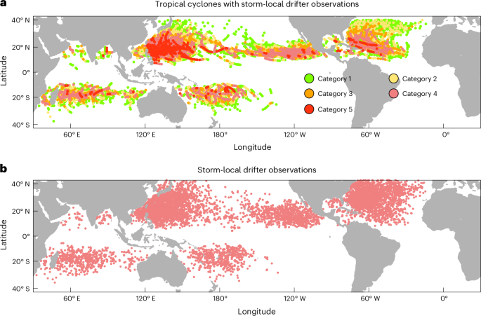
The Drifter Data Assembly Center at the Atlantic Oceanographic and Meteorological Laboratory applies quality control procedures to edit the position and SST observed by drifters and then interpolates them to 6-hour intervals. To determine TC-induced storm-local SST cooling, we search for paired pre-TC SST observations and then subtract them from storm-local SST observations. Detailed criteria are listed: (1) the storm-local SST should be observed at the exact time of TC passage within 500 km of the TC centre; (2) to calculate the storm-local SST cooling (that is, storm-local SST minus the reference pre-TC SST), the pre-TC SST observed 4 to 10 days before TC passage is identified to pair with the storm-local SST; (3) the distance between the paired storm-local SST and pre-TC SST observations should be less than 100 km to minimize the effect of background spatial ocean variability56. On the basis of the criteria, 32,801 storm-local SST and cooling observations are identified. Distribution of these storm-local drifter observations captures distribution of global TCs.
Following similar criteria to identify storm-local cooling, TC-induced SST cooling from 5 days before TC passage to 5 days after is further estimated based on drifter observations. We characterize the TC-induced SST cooling through composite analyses. SST cooling data, located within 100 km of TC centres, are averaged to obtain the temporal evolution.
We use different upper-bound distances of 50 km and 150 km to determine the TC-induced SST cooling for composite analyses. The results are consistent with that obtained using the upper-bound distance of 100 km (Extended Data Fig. 2a). Although we impose a limit on the pairing distance between storm-local SST and pre-TC SST, if the instrument crosses a mesoscale ocean feature, such as an eddy, with differing thermal features, the SST cooling could be affected. To examine the potential impact, we add a Lagrangian approach and a current velocity criterion to test the sensitivity of the cooling estimate. In the Lagrangian approach, we limit the TC-perturbed SST and the paired pre-TC SST observations to those measured by the same drifter. The composite result agrees with that obtained without this limitation (Extended Data Fig. 2b). Considering pre-existing mesoscale eddies potentially induce geostrophic current anomaly, we divide the SST cooling into two groups: with fast (> 0.3 m s−1) or slow (< 0.3 m s−1) currents accompanying the pre-TC SSTs. The 0.3 m s−1 is a mean pre-TC current velocity. Average SST cooling with fast or slow currents is consistent and agrees well with the cooling without a current limit criterion (Extended Data Fig. 2c). These results suggest that the impacts of mesoscale processes in the composite analysis are negligible.
Daily-averaged cooling by averaging 6-hourly drifter observations to comply with the daily microwave satellite and model output is −0.67 ± 0.02 °C, consistent with that based on 6-hourly observations (−0.68 ± 0.04 °C). This is probably because TC passage times are uniformly distributed (before or after) relative to satellite observations on day_0. Thus, when we compose the cooling based on a large number of samples, the impact of temporal inconsistency is filtered out.
SST in TC-active regions
TC-active regions refer to the areas where climatological SST exceeds 27 °C during TC seasons, excluding the equatorial band (5° N–5° S), the South Atlantic and the southeastern Pacific due to rare TC activities. The TC season is defined as August–October for the northern hemisphere and February–April for the southern hemisphere. Monthly SST from the Ocean Reanalysis System 5 (ORAS5, 0.25° × 0.25°), European Centre for Medium-range Weather Forecasts (ECMWF) Reanalysis v5 (ERA5, 0.25° × 0.25°), Extended Reconstructed Sea Surface Temperature (ERSST, 2° × 2°) and Hadley Centre Sea Ice and Sea Surface Temperature (HadISST, 1° × 1°) datasets, are employed to calculate the warming trend in TC-active regions. Reasonably changing the TC-active regions and TC seasons does not affect the SST trend or our major conclusions. For instance, the TC-active regions and TC seasons selected in the literature2 are tested and yield similar results.
Linear trend detection
The trend analyses are based on normalized values, calculated by subtracting an average value within each basin, following a method described in the literature9,10. By doing so, the influence of intra-basin changes on the global trend is isolated. Linear trend analyses are conducted using ordinary least-squares regression based on the 3-year running average data.
Sensitivity tests are conducted to assess the trend analysis. We reduce drifter samples, keeping the number of samples the same each year and repeat this process 10,000 times. No notable difference is identified. Moreover, we randomly resample the gridded Ocean Reanalysis System 5 (ORAS5) SST data according to drifter observations, repeating this process 10,000 times; and then compare the linear trend of the TC-active regional mean SST from these resamples with that from gridded ORAS5 SST data. A consistent linear trend of the tropical mean SST is identified.
Although a radius of 500 km is a larger area than TCs’ inner-core area and there is substantial spatial variability in the storm-local SSTs, it has little influence on the conclusion about the fast-warming storm-local SST trend. We calculate the storm-local SST warming trends using SSTs within 500 km, 300 km and 100 km from TC centres. In these cases, we observed a consistently fast-warming trend. We choose a radius of 500 km to include SST observations beneath TCs as much as possible.
Potential intensity
Potential intensity (PI) is the maximum intensity that a TC can achieve under given SST and atmospheric conditions37,38,57. In this study, PI is calculated based on the storm-local SST,
$${V}_{\mathrm{PI}}^{\,\,\,\,2}=\frac{\mathrm{SST}-{T}_{0}}{{T}_{0}}\frac{{C}_{\kappa }}{{C}_{{\rm{D}}}}({\kappa }^{\ast }-\kappa )$$
(1)
where \(\mathrm{SST}\) is the storm-local SST, \({T}_{0}\) is the outflow temperature, \({C}_{\kappa }\) is the dimensionless enthalpy transfer coefficient, \({C}_{{\rm{D}}}\) is the drag coefficient, \({\kappa }^{\ast }\) is the enthalpy of the ocean surface and \(\kappa\) is the enthalpy of the atmosphere near the surface. The outflow temperature and \({C}_{{\rm{D}}}\) are determined using the published code calculating the potential intensity (ftp://texmex.mit.edu/pub/emanuel/TCMAX/). Specifically, by using sounding data (temperature, humidity and pressure as functions of altitude), the equilibrium level where the parcel becomes cooler and denser than the surrounding environment and stops rising can be calculated; then the outflow temperature can be determined by averaging the temperatures at and above the equilibrium level. The ratio of \({C}_{\kappa }\) to \({C}_{{\rm{D}}}\) of 0.9 is used.
To calculate TC potential intensity, 6-hourly mean sea-level pressure, air temperature and specific humidity, at 19 isobaric levels (that is, 1,000; 950; 900; 850; 800; 750; 700; 650; 600; 550; 500; 450; 400; 350; 300; 250; 200; 150 and 100 hPa) are used. To ensure consistency with the drifter SST observations, they are interpolated to match the location of drifter SST observations.
PI-derived intensity trend
Following the method proposed in ref. 6, the theoretically expected mean intensity trend of Category 1–5 TCs based on PI trend, is explored. Assuming that PI can be described by an autoregressive process with autocorrelation coefficient \(r\), annual mean \(\mu\), standard deviation \(\sigma\) and an increasing trend \(\delta\), PI can be formed as
$$\mathrm{PI}(t)=\mu +\sigma x(t)+\delta (t)$$
(2)
$$x(t)=rx(t-\varDelta t)+\sqrt{1-{r}^{2}}\varepsilon (t)$$
(3)
where \(x\) is a standardized variable with zero mean and standard deviation of unity, \(r\) is the lag-1 (\(\varDelta t\)) autocorrelation, and \(\varepsilon\) is the white noise. For Category 1–5 TCs, assuming that TCs have a uniform probability of achieving any mean TC intensity between the minimum Category 1 intensity (that is, 33 m s−1) and the upper-bound intensity that TCs can achieve (that is, PI), synthetic time series of mean TC intensity can be formed as
$$\mathrm{Intensity}(t,\gamma (t))={\mathrm{Intensity}}_{\min }+(PI(t)-{\mathrm{Intensity}}_{\min })\gamma (t)$$
(4)
where \({\mathrm{Intensity}}_{\min }\) = 33 m s−1 and \(\gamma (t)\) is the random number drawn from a uniform distribution on the interval (0, 1). For each year, the number of \(\gamma (t)\) is a random number drawn from a Poisson distribution with the specified rate (global annual number of Category 1–5 TCs, approximately 49). To calculate the trend of mean TC intensity, we use the trend of the mean of the 10,000 subsamples for that expected trend. More details on this idealized experiment can be found in the literature6.
Comparing microwave satellite data with drifters
On the basis of drifter observations, we assess the uncertainties of TC-induced storm-local SST cooling observed by microwave satellites. Daily microwave optimally interpolated SST data version 5.0 from Remote Sensing Systems, with roughly 25-kilometre resolution, are used. Because this dataset has been available since 1998, we compare drifter and microwave satellite observations of TC-induced SST cooling from 1998 to 2021.
Although satellite microwave radiometers measure sub-skin SST at several millimetres beneath the surface influenced by diurnal warming, the sub-skin SSTs have been converted to foundation SSTs without diurnal warming by using a diurnal warming model41. Moreover, the upper ocean from the sea surface to O (100 m) depth is well mixed due to TC-induced strong turbulent vertical mixing17,19,24. Therefore, the difference in measuring depth between microwave satellites and drifters has a negligible influence on SST measurements under TC conditions.
By interpolating the gridded microwave SSTs to the locations of all drifter samples using bilinear interpolation, we obtain the projected microwave satellite observations to calculate the TC-induced SST cooling. Therefore, the comparison of composites between drifter and projected microwave satellite data is based on one-to-one paired data from the same TCs.
TC-induced SST cooling is further calculated based on gridded microwave satellite observations. When comparing the composites derived from projected and gridded microwave satellite observations, we find no noticeable difference between them (Extended Data Fig. 4). The result suggests that the composite TC-induced SST cooling derived from drifter and projected satellite observations is statistically robust.
We test the overestimation of inner-core SST cooling by microwave satellite data using independent moored buoys (and floats) in global TC-active basins. To identify inner-core SST cooling and maximize sample size, we pair each buoy with tropical depressions and tropical storms within 100 km and Category 1–5 within 500 km from TC centres that passed within the open ocean. In total, 2,078 storm-local observations from 55 buoys that encountered TCs are obtained, sourced from: the global tropical moored buoy array (Tropical Atmosphere Ocean Project, TAO/TRITON; Prediction and Research Moored Array in the Tropical Atlantic, PIRATA; Research Moored Array for African-Asian-Australian Monsoon Analysis and Prediction, RAMA); the National Data Buoy Center buoys; the floats under hurricanes Irma (2017) and Florence (2018); a G2 buoy that deployed in the South China Sea; the Kuroshio Extension Observatory (KEO) buoy; and the Bailong buoy under TC Dahlia (2017).
Enthalpy flux
Total enthalpy flux (\({Q}_{{\rm{t}}}\)), that is, sensible (\({Q}_{{\rm{s}}}\)) plus latent (\({Q}_{{\rm{l}}}\)) heat flux, is estimated using bulk aerodynamic formulas15,
$${Q}_{{\rm{s}}}={\rho }_{{\rm{a}}}{C}_{\mathrm{pa}}{C}_{{\rm{H}}}V({T}_{{\rm{s}}}-{T}_{{\rm{a}}})$$
(5)
$${Q}_{{\rm{l}}}={\rho }_{{\rm{a}}}{L}_{\mathrm{va}}{C}_{{\rm{E}}}V({q}_{{\rm{s}}}-{q}_{{\rm{a}}})$$
(6)
$${Q}_{{\rm{t}}}={Q}_{{\rm{s}}}+{Q}_{{\rm{l}}}$$
(7)
where \({\rho }_{{\rm{a}}}\) is the air density; \({C}_{{pa}}\) is the specific heat of air at constant pressure; \({L}_{\mathrm{va}}\) is the latent heat of vaporization at a given \({T}_{{\rm{a}}}\); \({C}_{{\rm{H}}}\) and \({C}_{{\rm{E}}}\) are the dimensionless coefficients of heat and moisture exchange, respectively, which are taken as 1.3 × 10⁻³ (ref. 58); \(V\) is the wind speed of TCs; \({T}_{{\rm{s}}}\) and \({T}_{{\rm{a}}}\) are the inner-core SST and near-surface air temperature respectively; \({q}_{{\rm{s}}}\) and \({q}_{{\rm{a}}}\) are the saturation mixing ratio at the inner-core SST and the actual mixing ratio of the air, respectively. In this work, the enthalpy flux is estimated using drifter SST observations and projected microwave satellite SST observations, respectively. Then, the enthalpy flux bias based on microwave satellite SST observations is estimated through a comparison with that based on drifter observations. Given that the wind speeds of TCs are generally spatially asymmetrical, the enthalpy flux calculated in this study, based on the maximum wind speed of TCs, may represent the upper bound of the spatial distribution of enthalpy flux.
Model simulations
Average inner-core SST cooling is evaluated in the HighResMIP experiments. The HighResMIP is an integral part of CMIP6, with the primary objective of enhancing the models’ capability by improving their horizontal resolutions. For each simulated TC centre, inner-core SST cooling is calculated within 100 km of TC centres on the day of TC passage.
In HighResMIP experiments, storm tracks from five models—Euro-Mediterranean Centre on Climate Change coupled climate model (CMCC-CM2), Centre National de Recherches Météorologiques model version 6 (CNRM-CM6-1), PRocess-based climate sIMulation: AdVances in high-resolution modeling and European climate Risk Assessment (PRIMAVERA) version of European Community Earth System Model (EC-Earth-3P), European Centre for Medium-Range Weather Forecasts-Integrated Forecasting System (ECMWF-IFS) and Hadley Centre Global Environmental Model 3—Global Coupled configuration 3.1 (HadGEM3-GC31)—are provided. These storm tracks are calculated using the ‘TRACK’ storm tracking algorithm59. The corresponding daily SST data are then utilized to calculate simulated inner-core SST cooling. Horizontal resolution of the SST data from HadGEM3-GC31 is 50 km, whereas that of the others is 25 km. We utilize the simulated data derived from historical experiments (hist-1950). Although the simulated data in the hist-1950 span from 1950 to 2014, we focus on the period between 1992 and 2014, covered by drifter observations.
The Coupled Ocean-Atmosphere-Wave-Sediment Transport Model (COAWST) modelling system consists of the Weather Research and Forecasting (WRF) as the atmospheric model, the Regional Ocean Modeling System (ROMS) as the oceanic model and the Simulating Waves Nearshore as the wave model. In this study, the WRF and ROMS coupling model are employed. Resolutions of both the WRF and ROMS models adopt identical grids with a horizontal resolution of 9 km. WRF has 39 vertical levels. Physical parameterization schemes in WRF include the Lin scheme for microphysics60, the Modified Tiedtke scheme for Cumulus convection61, the University of Washington scheme for the planetary boundary layer62 and the Monin–Obukhov (Janjic) scheme for the surface layer63. The ROMS model has 40 vertical levels. The Mellor–Yamada vertical mixing scheme is used in the simulation. By using the Model Coupling Toolkit, the exchange of environmental data between WRF and ROMS is achieved. The WRF and ROMS coupling model has been widely used for TC simulations12,54.
We simulate 22 TC cases for control runs, comprising 486 6-hourly recorded track points across Category 1–5 in the WNP. The simulation generates approximately 2,000 hourly model outputs. For experimental runs, we re-forecast these TCs with a reduced inner-core SST cooling for the ocean component of the modelling system. We reduce inner-core SST cooling by reducing vertical mixing, which dominates TC-induced SST cooling24, with all other conditions remaining unchanged. By comparing inner-core SST cooling and TC intensity between the control and experimental runs, we can isolate the effect of overcooling on TC intensity simulations. Uncertainty analysis is carried out using the Monte Carlo method12.
Overcooling in CMIP6 high-resolution models
Our analysis compares aggregated attributes from all observed TCs against those from thousands of TCs in climate models. In this regard, the impact from inter-event differences in TC attributes can be virtually averaged out, except for that from the underestimated TC intensity in the climate models, because it is a common bias. Despite the underestimation of modelled TC intensity, cooling is overestimated. The overcooling by models would probably be even more pronounced if the models were capable of reproducing higher TC intensities as observed in nature. Limited by this overcooling, and other factors such as low model resolution and uncertainties in model physics and parameterizations64,65, climate models can hardly reproduce intense TCs as observed.
As such, we use Category 1 TCs located in the WNP TC main development region for a comparison. Four of five models (except a few Category 1 TCs in the EC-Earth3P model) reproduce track densities of Category 1 TCs as those in best track records with drifter observations (Extended Data Fig. 8a–f). These climate models also reproduce translation speeds of TCs. In CMCC-CM2, CNRM-CM6-1 and HadGEM3-GC31, the average translation speeds of simulated TCs are consistent with observations in the best-track dataset, with a small bias of no more than 0.08 m s−1. One exception is that the ECMWF-IFS model produces TCs with a faster average translation speed (6.98 m s−1) than that of best-track TCs (5.12 m s−1). However, this faster translation speed in the ECMWF-IFS model should have resulted in less cooling than observations, but the overcooling is still produced. Thus, under the same TC intensity (Category 1), these models produce an overestimate of the TC-induced cooling, statistically significant above the 95% confidence level (Extended Data Fig. 8g). The multi-model ensemble mean for slow TCs shows a more than 80% overestimate, and for fast TCs, there is an overestimate of about 150%. We further analysed the cooling bias under different TC intensities in the WNP main development region using output from the CNRM-CM6-1 model. This model is selected because it successfully simulates TCs from Tropical Depression to Category 4, while other models fail to simulate Category 3–5 TCs. We find that overcooling consistently occurs for individual TC intensities (Extended Data Fig. 8h).