
Study area and data collectionAdministrative dataset
In this study, we included a total of 180 countries using the World Bank’s Global Administrative Divisions data49. This dataset classifies the world into seven regions: North America, Europe & Central Asia, East Asia & Pacific, Latin America & Caribbean, Middle East & North Africa, South Asia, and Sub-Saharan Africa (Fig. S1a), as well as four income groups: low income, lower-middle income, upper-middle income, and high income (Fig. S1b). We also incorporated county-level administrative boundaries from the GADM database50, covering over 30,000 counties (Fig. S1c).
CHAT dataset
We used the Cross-country Historical Adoption Technology (CHAT) dataset51, an aggregation of country-level statistics sourced from national income accounts and various multilateral agencies. The CHAT dataset contains annual information on technology use for 161 countries from 1820 to 2003, encompassing 104 technologies across sectors, such as transportation, communication and IT, industrial, agricultural, and medical.
Climate data
We derived global annual mean temperature, cumulative precipitation, and cumulative evapotranspiration for the period 1980–2023 from the TerraClimate dataset52, which provides monthly climate and climatic water balance variables for global terrestrial surfaces at a 5-km spatial resolution. Specifically, annual mean temperature was calculated as the average of monthly minimum and maximum temperatures (from the ‘tmmn’ and ‘tmmx’ bands). Cumulative precipitation and evapotranspiration were obtained from the ‘pr’ and ‘aet’ bands, respectively.
Cropland data
We used the global dynamic cropland data from Potapov, Turubanova53 to estimate worldwide cropland areas. Cropland was mapped every four years (2000–2003, 2004–2007, 2008–2011, 2012–2015, and 2016–2019) at 30 m spatial resolution to minimize the impact of fallow cropland on classification. We selected this dataset due to its rigorous validation process and higher accuracy compared to other globally available cropland datasets. Also, it has been shown to align well with FAO cropland statistics54. For our analysis, we used the most recent 2019 cropland layer to represent the available cropland extent for ERW. Within each 5 × 5 km grid cell, the total cropland area was computed using the Google Earth Engine platform55.
Future global warming data
The SSP database is a comprehensive resource that offers data on projected global socioeconomic and environmental changes under different SSPs. These pathways explore a range of potential futures related to global development, climate change mitigation, and adaptation. For our analysis, we extracted the GCAM4-SSP4 baseline warming data from 2010 to 2100 with a 10-year interval from the SSP database.
Projection of future ERW adoption shares
We used the theoretical approach of Comin and Hobijn28 to simulate the historical diffusion of technologies, where the estimating equation is constructed from a one-sector growth model in the context of endogenous total factor productivity differentials:
$${{Ln}(Y)}_{i,t}={\beta }_{1,i}+{\beta }_{2}t+{\beta }_{3}{ln}\left(t-{D}_{i}\right)-0.7{\beta }_{3}\left(\frac{{{GDP}}_{i,t}}{{{Pop}}_{i,t}}\right)+{\epsilon }_{i,t}$$
(1)
where the dependent variable Yit captures the physical measure of technology adoption for a given technology at time t for country i (i.e., irrigated area, fertilizer use, or number of harvesters). The intercept β1i represents the country-technology fixed effect, which absorbs the cross-country differences in total factor productivity and the relative prices of capital. Meanwhile, β2 is the trend parameter universal for all countries since it only depends on the output elasticity of capital. Similarly, β3 is technology-specific but is constant across countries. The last term is negative, because it represents the competing trade-offs between capital and labor in the production process and is scaled by the output elasticity of labor (0.7). Another key empirical parameter is the adoption lag, Di, the time between invention and initial take-up. A larger Di would suggest that a long time ago, the lead innovator (e.g., the United States) had already exhibited the same level of adoption intensity in country i.
Additionally, we included GDPit and Popit in Eq. (1) to account for annual gross domestic product and population, respectively, as controls for economy-wide conditions. The intensity of technology adoption is an endogenous decision influenced by capacity constraints, including access to capital, labor skill composition, and complementarity of the new technology to the existing production process. Hence, the income term (GDP/Pop) serves as an approximation of these critical factors.
While the CHAT dataset includes diffusion pathways for more than one-hundred technologies across various sectors, we focused on a few relevant agricultural innovations (i.e., fertilizers, harvesters, and irrigation; Table S1) to develop analogs for the region-specific ERW adoption curves. Fig. S2 presents time series data and fitted diffusion curves for these technologies in selected countries. The fitted diffusion trajectories estimated from Eq. (1) were then normalized to ensure comparability across technologies and regions using the following transformation:
$$\hat{{y}_{t}}={Ceiling}\times \frac{{Y}_{t}-{Y}_{min }}{{Y}_{max }-{Y}_{min }}$$
(2)
where \(\hat{{y}_{t}}\) represents the normalized adoption share at time t (in percentage) derived from the historical diffusion trajectory of the representative analog technology, and Ymin and Ymax denote its minimum and maximum observed values within the historical record. Ceiling is a predefined upper limit of adoption (e.g., 50% or 75%) representing different levels of policy and behavioral ambition. These adoption ceilings are consistent with ranges reported in the existing ERW literature2,16. This normalization preserves the relative curvature and lag structure of each analog while scaling them to a common adoption range defined by the scenario-specific ceiling.
In practice, we extrapolated the annual adoption trajectories of ERW across regions using parameters estimated from Eqs. (1–2), letting t start from 2025 and extending to 2100. Due to the limited number of observations, many country-scale regression models were not statistically significant. Consequently, we modeled technological diffusion at a broader regional scale, covering seven global regions (Fig. S1a). For each region, we selected the curve that best fits the data with the highest R² value among the three technologies considered. Table S2 summarizes the selected technology and corresponding model performance for each region, and Fig. S3 compares the modeled and observed adoption trajectories of these analog technologies. Further illustrations of model implementation, accuracy, and robustness tests are available in the Supplementary Materials.
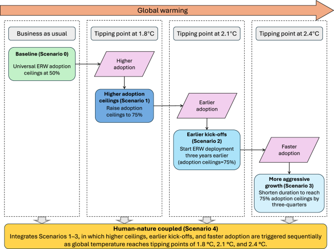
In addition to the adoption growth developed from historical analogs, we set the maximum adoption shares (e.g., a 50% ceiling for ERW in the baseline scenario) to be more conservative. We also adjusted the model parameters (e.g., raising the adoption ceilings to 75% in Scenario 1) for each scenario considered in this study. Detailed descriptions of the scenario settings are provided in the Supplementary Materials.
Estimation of carbon sequestration rate
The CDR potential of ERW is modified by multiple biophysical factors, particularly temperature and soil excess water (i.e., annual precipitation minus actual evapotranspiration). In general, higher soil temperature and excess water enhance carbon sequestration through accelerated weathering rates56,57. In this study, we estimated the annual carbon sequestration rate of ERW as the mean value for the 1980–2023 period at a 5-km spatial resolution using the following equation:
$$K\left(T,E\right)={K}_{0}\times f(T)\times f(E)$$
(3)
where K(T,E) is the annual carbon sequestration rate under specific temperature (T) and water surplus (E) conditions. K0 is a baseline carbon sequestration rate under reference soil temperature and water conditions. Here we assumed K0 to be 1.5 tCO2 ha-1 yr-1. This number is a relatively conservative estimate of the potential of CDR under moderate ERW application (i.e., 10 tons ha-1 Olivine or equivalent silicate minerals application) after considering constraints from soil biogeochemical properties57,58, which is held constant across all scenarios and regions in the diffusion model. f(T) and f(E) are two scaling functions that represent the modifying effects of temperature and water availability on weathering kinetics, and can be expressed as:
$$f\left(T\right)=exp \left[-\frac{{E}_{a}}{R}(\frac{1}{T}-\frac{1}{{T}_{0}})\right]$$
(4)
$$f\left(E\right)=\left\{\begin{array}{c}0,E\le {E}_{p10}\,\\ \frac{E-{E}_{p10}}{{E}_{p90}-{E}_{p10}},{E}_{p10} < E\le {E}_{p90}\\ 1,E > {E}_{p90}\end{array}\right.$$
(5)
Here, Ea = 70,500 J mol-1 is the activation energy for silicate weathering59, R = 8.3145 J mol-1k-1 is the universal gas constant, and T0 = 288.15 K (15 °C) is the reference temperature. The temperature function f(T) captures the Arrhenius dependence of weathering reactions, with higher temperatures accelerating carbon sequestration. This equation has been verified by previous literature in representing the temperature dependence of rock weathering kinetics2,60. The soil water surplus function f(E) is modeled as a piecewise linear response modified from Houlton, Morford56, where E is the annual water surplus, calculated as the difference between precipitation (PR) and actual evapotranspiration (AET). The thresholds Ep10 and Ep90 (set at 23.61 mm yr-1 and 607.24 mm yr-1, respectively) denote the 10 and 90th percentiles of global water surplus distribution. Below Ep10, ERW is constrained by insufficient moisture, while above Ep90, water is no longer a limiting factor. Fig. S4 shows the response curves for f(T) and f(E) and Fig. S5 displays the estimated global carbon sequestration rates on croplands.
This biophysically informed modeling framework allows us to spatially differentiate ERW carbon removal potential under heterogeneous climatic conditions, providing a robust basis for identifying geophysical hotspots suitable for deployment.
Quantification of ERW’s CDR
Building on both societal adoption dynamics and biophysical suitability, we estimated the annual CO2 removed by ERW for each 5-km × 5-km grid cell using the following approximation:
$${{CO}}_{2}\left(k,t,s\right)={A}_{k,t,s}\times {K}_{k}\times {L}_{k}$$
(7)
where CO2 (k,t,s) is the annual CO2 sequestration for grid k in year t under scenario s. Ak,t,s refers to the ERW adoption share for grid k in year t under scenario s, modeled based on Eqs. (1–2). Kk is the CO2 sequestration rate (tCO2 ha-1 yr-1) for grid k under specific temperature (T) and water surplus (E) conditions (Eq. (3)). Lk is the total cropland area for grid k, derived from the GLAD cropland data.
For our human-nature coupled model (Scenario 4), we adapted the above equation to dynamically respond to diverse global temperature tipping points (TP), indicating societal responses to a warming climate.
$${{CO}}_{2}\left(k,t,s4\right)=\left\{\begin{array}{c}\begin{array}{c}{A}_{k,t,s0}\times {K}_{k}\times {L}_{k},\hfill{if\; TP} < 1.8{{^{\underline{{\rm{o}}}} }}C \\ {A}_{k,t,s1}\times {K}_{k}\times {L}_{k}, \qquad{if}1.8{{^{\underline{{\rm{o}}}} }}C\le {TP} < 2.1{{^{\underline{{\rm{o}}}} }}C \\ {A}_{k,t,s2}\times {K}_{k}\times {L}_{k}, \hfill{if}2.1{{^{\underline{{\rm{o}}}} }}C\le {TP} < 2.4{{^{\underline{{\rm{o}}}} }}C\end{array}\\ {A}_{k,t,s3}\times {K}_{k}\times {L}_{k}, \hfill{if}\; {TP} > 2.4{{^{\underline{{\rm{o}}}} }}C\end{array}\right.$$
(8)
The changes in subscripts represent transitions triggered when specific warming thresholds (i.e., 1.8 °C, 2.1 °C, 2.4 °C) are crossed. The adoption shares Ak,t,0, Ak,t,1, Ak,t,2, and Ak,t,3 reflect the shifts in the proportion of croplands allocated to ERW, which capture the influence of societal adaptation and policy incentives in response to increasing global temperatures. These adoption shares describe how the proportion of cropland allocated to ERW increases as warming intensifies. The underlying assumption is that more severe climate impacts heighten public risk perception, accelerate social learning, and increase policy support for mitigation—mechanisms widely documented in behavioral and environmental social science22,23. In this way, the model reflects how worsening climate conditions could stimulate faster ERW deployment, consistent with prior work emphasizing the need to couple human behavior with Earth-system feedback to better represent real-world mitigation potential29,30,31,32,33.
We chose Shared Socioeconomic Pathway 4 (SSP4) as our baseline climate scenario to represent background temperatures from the present to 2100. This pathway is characterized by inequality, where disparities between regions and within countries are prominent61. In SSP4, a small group of highly developed, technologically advanced countries can adopt and implement mitigation technologies at a much faster rate, while a larger portion of the world, particularly developing countries, faces pronounced barriers to technological diffusion and economic growth. Accordingly, the choice of SSP4 aligns with our objective of projecting the unequal spatial and temporal paces of ERW adoption across regions and its implications for future climate change. Practically, annual increases in global temperatures were interpolated via linear regression analysis on the GCAM4-SSP4 baseline warming with a 10-year interval from the SSP database62.
To assess long-term CDR potential, we computed the cumulative CO₂ sequestration of ERW from the base year 2025 through year t using the following equation:
$${Cum}{{CO}}_{2}\left(k,t,s\right)={\sum }_{j=2025}^{t}{{CO}}_{2}\left(k,j,s\right)$$
(9)
where CumCO2 (k,t,s) represents the cumulative CO2 sequestration for grid k by year t under scenario s. These values were further aggregated to both country (Fig. 5) and county (Fig. S6) levels to reveal regional disparities in ERW’s CDR potential.
Sensitivity analysis
We performed three additional analyses to evaluate the sensitivity of our results and assess how these assumptions influence global CDR potential from ERW. First, we introduced a supplementary scenario with a 25% adoption ceiling, representing a conservative lower bound of ERW diffusion. Second, we considered future cropland dynamics in the computation of CDR potential using gridded cropland projections from Ref63., which provide estimates of cropland proportions through 2100 under various SSP–RCP scenarios. In this implementation, Lk in Eq. (7) was calculated based on the available cropland in each year under the corresponding climate scenario. We selected SSP4–RCP3.4 and SSP4–RCP6.0, consistent with the SSP4 framework adopted in this study. Third, to assess the robustness of our findings to alternative climate policy environments, we conducted a sensitivity test by rerunning Scenario 4 under the SSP4–RCP6.0 pathway, which incorporates moderate climate policy and yields lower global warming. Under this trajectory, reduced climatic stress leads to a weaker human–nature response and correspondingly lower global ERW adoption and cumulative CDR (Figs. S9–S10). Nevertheless, the spatial and temporal patterns of adoption remain broadly consistent with those under the SSP4 baseline (Fig. 3). This analysis indicates that although the magnitude of ERW deployment is sensitive to the underlying warming scenario, the qualitative patterns and regional ordering of adoption are robust across contrasting socioeconomic–climate baselines.