
The workspace and equipment in the pre-PCR area were sterilised with hypochlorite solution before library preparation. Low-retention filtered pipette tips and microtubes were used and pre- and post-PCR manipulations were performed in two different dedicated rooms to safeguard against carryover contamination. Two-step PCR (first-round PCR and index PCR) was applied for paired-end next generation sequencer (NGS) library preparation, following previously developed methods43,44. For the first-round PCR (1st PCR), a mixture of two primer pairs was used: MiFish-U-forward (5′–ACA CTC TTT CCC TAC ACG ACG CTC TTC CGA TCT NNN NNN GTC GGT AAA ACT CGT GCC AGC–3′), MiFish-U-reverse (5′–GTG ACT GGA GTT CAG ACG TGT GCT CTT CCG ATC TNN NNN NCA TAG TGG GGT ATC TAA TCC CAG TTT G–3′), MiFish-E-forward-v2 (5′–ACA CTC TTT CCC TAC ACG ACG CTC TTC CGA TCT NNN NNN RGT TGG TAA ATC TCG TGC CAG C–3′) and MiFish-E-reverse-v2 (5′–GTG ACT GGA GTT CAG ACG TGT GCT CTT CCG ATC TNN NNN NGC ATA GTG GGG TAT CTA ATC CTA GTT TG–3′). The 1st PCR was carried out with a 12-µl reaction volume in eight replications using a strip of eight 0.2-ml tubes. A 1st PCR blank (1B) was also prepared during this process. To reduce the experiment costs, a single 12-µl reaction was prepared for each type of blank (FB, EB, and 1B). After the 1st PCR, equal volumes of the PCR products were pooled from the eight replications in a single tube and purified using a GeneRead Size Selection Kit (Qiagen, Hilden, Germany). Subsequently, the purified target products (ca. 300 bp) were quantified using TapeStation 2200 (Agilent Technologies, Tokyo, Japan). After diluting samples to 0.1 ng/µl with Milli-Q water, 1.5 µl of each diluted product was subjected to the index PCR (2nd PCR) in a 12-µl reaction volume to append dual-indexed sequences and flow cell-binding sites for NGS platform. For the three types of blanks (FB, EB, and 1B), the 1st PCR products were purified in the same manner but were not quantified. They were diluted at the average dilution ratio of the positive samples to be used as templates for the 2nd PCR. The following two primers were used for the 2nd PCR to append dual-indexed sequences (eight nucleotides indicated by Xs) and flow cell-binding sites for the MiSeq platform (5′–ends of the sequences before eight Xs): 2nd-PCR-forward (5–AAT GAT ACG GCG ACC ACC GAG ATC TAC ACX XXX XXX XAC ACT CTT TCC CTA CAC GAC GCT CTT CCG ATC T–3′) and 2nd-PCR-reverse (5′–CAA GCA GAA GAC GGC ATA CGA GAT XXX XXX XXG TGA CTG GAG TTC AGA CGT GTG CTC TTC CGA TCT–3′). A 2nd PCR blank (2B) was made during this process.
To monitor contamination during on-site filtration, DNA extraction, and 1st and 2nd PCRs, 321 blanks were made (FB = 191, EB = 52, 1B = 65, 2B = 13) and subjected to the library preparation procedure. They were divided into four sets and the libraries were pooled in equal volumes into four 1.5-ml tubes. The target amplicons (ca. 370 bp) were purified using a 2% E-Gel Size Select agarose gel (Invitrogen, Carlsbad, CA). The concentration of the size-selected libraries was measured using a Qubit dsDNA HS Assay Kit and a Qubit fluorometer (Life Technologies, Carlsbad, CA), diluted to 12.0 pM with HT1 buffer (Illumina), and sequenced on the MiSeq platform (Illumina, San Diego, CA) using a MiSeq v2 Reagent Kit, 300 cycles (Illumina) with a PhiX Control v3 (Illumina, San Diego, CA) spike-in (expected at 5%), following the manufacturer’s protocol. To remove residual contamination from the MiSeq flow path, the flow channel was washed with hypochlorous acid before each operation. All raw DNA sequence data and associated information were deposited in DDBJ/EMBL/GenBank (accession number DRA007474).
Data preprocessing and taxonomic assignment
Data preprocessing and analyses were performed using MiSeq raw reads from the 528 samples. Using USEARCH ver. 10.0.24045, quality-filtered forward and reverse reads were merged, primer sequences were removed, low-quality reads were filtered, and reads were dereplicated and denoised to obtain amplicon sequence variants (ASVs). Finally, fish species (molecular operational taxonomic units; MOTUs) were assigned to ASVs with a sequence identity of > 80% with the reference sequences. A custom reference database (see details in Supplementary Information S1) was used. Four expert ichthyologists (M.M., H.Motomura, T.Sado, and H.S.) revised the taxonomic assignments based on phylogenetic relationships combined with their knowledge of species distributions and dominance. The details of data processing, database assembly, and taxonomic assignment are described in Supplementary Information S1.
To focus on coastal fishes, all fishes principally inhabiting regions outside of the coastal areas (deep-sea fishes, oceanic epipelagic fishes, pure freshwater fishes, and all non-native fishes originating from food materials and carryover contamination) were excluded (Supplementary Table S2). Read counts were subsequently rarefied to the approximate minimum numbers (Supplementary Table S3).
Collecting environmental covariates
To reduce the burden of fieldwork, only seawater temperature and salinity were measured at each site after water sampling and on-site filtration. Additionally, four environmental covariates were collected from publicly available satellite data46: annual minimum and maximum sea surface temperatures in 2017, mean chlorophyll a concentration in June-August 2017 and mean particulate inorganic carbon concentration in June-August 2017. The resolution of all collected satellite data is 4 km × 4 km. The field-measured seawater temperature and salinity were missing at ten sites due to instrument failure. Therefore, data from these sites were removed from the subsequent analysis. Furthermore, the following MOTU data were removed: (1) MOTUs categorised as species complex (i.e. including several species) and (2) MOTUs occurring at fewer than six sites. Consequently, the subsequent analyses included 519 species from 518 sampling sites.
Nonlinear multivariate analysis
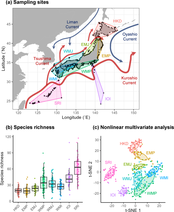
To better understand the regional community structure, sampling sites were geographically grouped into eight districts based on commonly used climate classifications and geographic proximity: Hokkaido Island (HKD, n = 71), East Main Island along the Pacific Ocean (EMP, n = 39), East Main Island along the Japan Sea (EMJ, n = 39), West Main Island along the Pacific Ocean (WMP, n = 95), West Main Island along the Japan Sea (WMJ, n = 90), West Main Island along inland sea (WMI, n = 63), Izu-Ogasawara Island (IOI, n = 51) and Satsuma-Ryukyu Island (SRI, n = 80). A nonlinear dimensionality reduction method, t-distributed stochastic neighbor embedding (t-SNE)47, was used to capture the structures of the entire regional fish community based on Jaccard distances between 518 sites.
Generalised linear latent variable model
Joint species distribution models are used to analyse co-occurrence patterns while accounting for missing predictors. In this study, a generalised linear latent variable model (GLLVM)7,8,9 with spatially autocorrelated latent variables (LVs) was used as a joint species distribution model to explore the hidden niche space. The GLLVM decomposes high-dimensional residual correlations using low-dimensional LVs, thus allowing fitting to relatively large datasets. The model structure was a logistic regression with environmental covariates (\(\:{\varvec{x}}_{\varvec{i}}\)) and spatially autocorrelated LVs (\(\:{\varvec{u}}_{\varvec{i}}\)) as explanatory variables and species presence-absence (\(\:{y}_{ij}\)) as response variables:
$$\:{y}_{ij}\:\sim\:\text{B}\text{e}\text{r}\text{n}\text{o}\text{u}\text{l}\text{l}\text{i}\left({p}_{ij}\right),\:\text{l}\text{o}\text{g}\text{i}\text{t}\left({p}_{ij}\right)={\beta\:}_{j0}+{\varvec{x}}_{i}^{\top\:}\:{\varvec{\beta\:}}_{j}+{\varvec{u}}_{i}^{\top\:}\:{\varvec{\gamma\:}}_{j}+{\alpha\:}_{i},$$
for fish species \(\:j\) = 1, …, 519 at sampling site \(\:i\) = 1, …, 518. \(\:{\varvec{\beta\:}}_{j}\) and \(\:{\varvec{\gamma\:}}_{j}\) are species-specific responses related to the environmental covariates and LVs, respectively. \(\:{\beta\:}_{j0}\) is the species-specific intercept and \(\:{\alpha\:}_{i}\) is random site effects. The random site effects can mitigate the bias owing to the variation in total eDNA concentrations among sites9. The spatial autocorrelation was modelled by Gaussian Markov random field48 (Supplementary Figure S4). The details of the model structure are described in Supplementary Information S2.
This study considered three candidate models with different sets of environmental covariates. As environmental covariates, Model (a) included the two field-measured variables, Model (b) included the four satellite variables and Model (c) included both the two field-measured variables and the four satellite variables. Furthermore, models with different numbers of latent variables (from 0 to 5) were also considered for each candidate model. Using five-fold cross validation with negative log-likelihoods as the validation loss, the Model (a) with three spatially autocorrelated LVs was selected as the best-fit model from 18 candidate models. In the main text, the results of this best-fit model were mainly reported for simplicity, whereas the results of the best-fit model of Models (b–c) were reported in Supplementary Information S2. Model (a) exhibited considerably higher model predictive ability for the regional fish community than Models (b–c) (Supplementary Table S5). Nevertheless, these models estimated similar geological variations in latent variables 1 and 2 and reproduced the five hypothetical biogeographic boundaries described in the following paragraph (Supplementary Figure S5).
As several previous studies49,50 did, our study defined biogeographic boundaries based on the ordination space (Fig. 2). Given that GLLVM directly relates ordination axes (i.e. latent variables) to species occurrence probabilities, community compositions are expected to change largely at the boundary of the zero-value line. Thus, zero-value lines were used to identify hypothetical biogeographic boundaries. The first and second LVs revealed five hypothetical boundaries between distinct local communities (Fig. 2 and Supplementary Figure S2). The third LV showed broad zero-value areas (not zero-value lines), suggesting no boundaries between communities (Supplementary Figure S2). Species niche centres were defined as the position with the highest occurrence probability in the niche space. For this, species occurrence records in geographic space were mapped onto the niche space and then the occurrence probability on the niche space was calculated using a kernel density estimation method.
Calculation of response diversity
To calculate the response diversity of a local community to each LV, 100 communities were randomly generated with estimated occurrence probabilities (\(\:\varvec{p}\)). The interquartile range of the response to each LV (\(\:\varvec{\gamma\:}\)) was calculated for the species comprising each generated community and the interquartile ranges over all 100 generated communities were averaged as the expected response diversity. The interquartile range was used instead of the other dispersion proxies (e.g. variance) to reduce the influence of outliers due to estimation error.
Spectral clustering and linear regression were used to investigate the relationship between species richness and response diversity. Local communities were classified into high and low expected response diversity using spectral clustering (the number of clusters was set to two). Then, linear regression was applied to each cluster:
$$\:\text{l}\text{o}\text{g}\left(response\:diversity\right)\:\sim\:\text{l}\text{o}\text{g}\left(richness\right).$$
To ensure homogeneity of variances, both species richness and response diversity were log-transformed. Because spectral clustering can produce several different results due to the randomness in the optimisation process, clustering was repeated 100 times and finally the clustering result with the highest log-likelihood was selected for linear regressions. All codes are available at https://doi.org/10.5281/zenodo.17823192.