
Concept of spin-orbit interactions driven by beam topology
Before demonstrating how topological structuring enables SOI in paraxial light, we briefly outline their origins in light-matter interaction. Optical SOI manifest when initially linearly polarized beams develop spatially varying spin, typically via interaction with dielectric surfaces, anisotropic and inhomogeneous media, or tight focusing. These processes produce spin-dependent beam shifts such as the Goos-Hänchen and Imbert-Fedorov effects33,34, and radial spin separation driven by orbital structure26, all arising from spin-orbit coupling13, as illustrated in Fig. 1a and b, respectively.
Fig. 1: Concept of spin-separation in vectorial fields.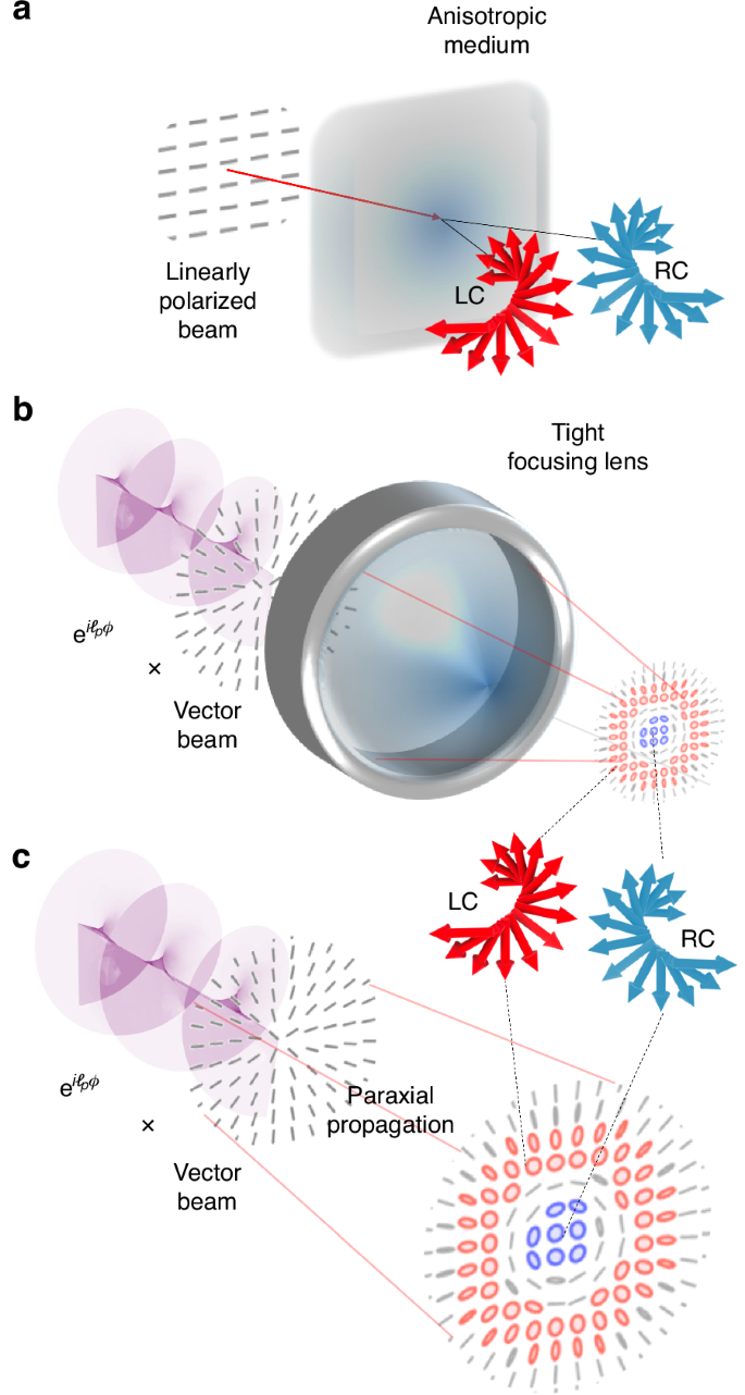 The alternative text for this image may have been generated using AI.
a Spin-dependent separation resulting from a vectorial field interacting with an anisotropic medium, therefore resulting in a photonic spin-Hall effect. Lateral transverse shifts are observed depending on the spin components of the incident field. b Spin separation induced by tight focusing of a radially polarized vectorial beam carrying a PT phase with a corresponding topological charge, ℓp, and (c) reproduced by propagating the same field but through free space without any interactions with matter. In each case, spin separation is observed in the evolved vector beam, showing regions dominated by right-handed and left-handed circular polarizations
Accordingly, these effects can also be viewed as being produced by polarization-dependent field gradients that separate spin components, akin to spin transport in electronic systems where electron spin-dependent flow and separation in the presence of an electric current can be observed14. As the spins separate spatially, two signatures emerge: (i) chiral spin textures with localized optical chirality (helicity), and (ii) spin currents characteristic of photonic spin-Hall effects. Here we show that by encoding topological structure into vector beams, these features can be realized in free-space within the paraxial regime – enabling spin separation and chiral spin flows without relying on strong focusing or complex media.
Topology-driven spin-orbit interactions in paraxial light
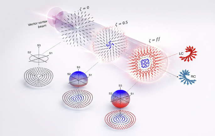
To generate SOIs that result in spin generation and separation within laser beams, one can tightly focus (see Fig. 1b) a scalar beam35,36,37 or vector vortex beam25,26,38,39,40,41,42,43,44,45,46,47 to produce so-called orbit-induced local spin (OILS). However, as we will demonstrate, these effects can also be realized in the paraxial regime, without the need for tight focusing. The approach begins with an optical field that exhibits a spatially varying linear polarization combined with a global azimuthal phase profile, as illustrated Fig. 1c. The corresponding electric field has the initial profile
$${{\bf{U}}}_{\rm{in}}({\bf{r}})\propto{\text{e}}^{i{\ell }_{p}\phi }\times \underbrace{{f}_{\rm{in}}({\bf{r}})({\rm{e}}^{i\Delta \ell \phi }{\hat{\sigma}}_{+}+{\rm{e}}^{-i\Delta \ell \phi }{\hat{\sigma}}_{-})}_{{\rm{radial}}\,{\mathrm{field}}}$$
(1)
in polar coordinates, r = (r, ϕ) with σ± representing the right and left CP, each marked with azimuthal phase profiles, \(\exp (\pm i\Delta \ell \phi )\) with \(\Delta \ell \in {\mathbb{Z}}\). At this point, it is crucial to notice that the polarization components each have the same radial amplitudes (fin( ⋅ )). The global phase, which has been factorized from the state, \(\exp (i{\ell }_{p}\phi )\) characterized by the PT index \({\ell }_{p}\in {\mathbb{Z}}\), encodes the elusive topological features that we are interested in as this controls the spin-orbit interactions in the field. Given the above electric field, the topological phase can be computed from (See Supplementary Material)
$${\phi }_{p}=\arg (\langle {{\bf{U}}}_{{\text{in}}}(0)| {{\bf{U}}}_{\text{in}}(\phi )\rangle )=\frac{{\ell }_{p}}{2}\phi$$
(2)
which is directly linked to the PT winding number that is also associated with the total OAM of the VVB (see Supplementary Material). Setting ℓp = 0 produces a typical radially polarized field that does not carry this phase (nor total OAM) and remains unchanged, i.e., maintaining the same polarization profile on propagation. However, for ∣ℓp∣ > 1 the field carries nonzero OAM while the PT phase causes the polarization field to change across the beam in the transverse plane on propagation, so that the new field maps as
$${{\bf{U}}}_{{\text{in}}}\to {\bf{U}}={f}_{{\ell }_{{\text{A}}}}({\bf{r}}){{\text{e}}}^{i{\ell }_{{\text{A}}}\phi }{\widehat{\sigma }}_{+}+{f}_{{\ell }_{{\text{B}}}}({\bf{r}}){{\text{e}}}^{i{\ell }_{{\text{B}}}\phi }{\widehat{\sigma }}_{-,}$$
(3)
where \({f}_{{\ell }_{{\text{A}}({\text{B}})}}({\bf{r}})\) represent the new field amplitude distributions for each spin component, that now depend on the PT charge, ℓA(B) = ℓp ± Δℓ, respectively. As a consequence, one observes that the spin components separate radially in the field. For example, in the output profile of the concept illustration in Fig. 1c, we see that close to the core (r ≈ 0), the field is dominated by right circular spins and subsequently dominated by left circular spins as one scans the field radially outward – a key signature of local spin generation – whereas initially the field had no local spin components. This can be measured by quantifying the local optical chirality density and longitudinal spin densities, which are both proportional to the third Stokes parameter (See Supplementary Material for the derivation), S341, i.e,
$${S}_{3}=| {f}_{{\ell }_{{\text{A}}}}(r,z){| }^{2}-| {f}_{{\ell }_{{\text{B}}}}(r,z){| }^{2}$$
(4)
that can be extracted from the transverse plane for various longitudinal coordinates, z. The third Stokes parameter can be measured experimentally via the difference in intensities between the space-dependent amplitudes marking each spin state. The reason for extracting the optical chirality C and spin density s from the Stokes parameter (S3) follows from the fact that in the paraxial regime, these quantities take familiar forms, with the spin being purely longitudinal; sz ∝ C ∝ σI, where σ is the helicity (for circular polarization σ = ± 1, for elliptical ∣σ∣ < 1, and for linear or unpolarized light σ = 0), and I is the beam intensity. We show that radial spin separation originates from amplitude symmetry breaking due to topological encoding, and elucidate its propagation dependence via S3 and the associated polarization profiles.
Inducing SOI in paraxial fields through topology-driven amplitude change in propagation
Now we uncover the mechanism that enables one to observe SOI in paraxial beams. Firstly, notice that the vector beams described by Eq. (3) are hybrid-order Poincaré beams (HyOPs) and are not eigenmodes of free-space propagation48 when ∣ℓp∣ > 0. As they propagate, the local states of polarization evolve along z due to differential Gouy phase shifts and radial amplitude variations between the constituent modes that mark the right and left CP states. This leads to a spin-dependent splitting into concentric rings, each carrying opposite circular polarization and different OAM – a signature of propagation-driven optical Hall effect. While hybrid-order vector beams are not eigenmodes of free-space propagation, this alone does not fix the form of the resulting spin density; here, its emergence is deterministically governed by the Pancharatnam topological index.
To demonstrate this in the paraxial regime, we prepared a scalar horizontally polarized Laguerre-Gaussian (LG) mode, as shown on the left of the concept image in Fig. 1c, having a characteristic field profile that can be expressed as
$${{\text{LG}}}_{{\ell }_{p}}({\bf{r}})\widehat{{\bf{x}}}={f}_{{\ell }_{p}}(r,z){{\text{e}}}^{i{\ell }_{p}\phi }\widehat{{\bf{x}}}$$
(5)
where \((\widehat{{\bf{x}}}={\widehat{{\boldsymbol{\sigma }}}}_{+}+{\widehat{{\boldsymbol{\sigma }}}}_{-})/\sqrt{2}\) and r = (r, ϕ, z) are the polar coordinates. The LG modes used here have a characteristic radial profile, \({f}_{{\ell }_{p}}(r,z)\propto {(\sqrt{2}r/w)}^{| {\ell }_{p}| }\exp (i({\psi }_{G}+kz)-{r}^{2}/{w}^{2})\) where w[z] is the waist size of the embedded Gaussian component of the field (\({{\text{e}}}^{-{r}^{2}/{w}^{2}}\)); a Gouy phase \({\psi }_{{\text{G}}}=(| {\ell }_{p}| +1)\arctan (z/{z}_{{\rm{R}}})\); and an azimuthal phase, \(\exp (i{\ell }_{p}\phi )\). Note how the topological charge determines the change in the Gouy phase term, as well as the divergence through the radial term. The resulting field will be modulated with a spin-orbit coupling (SOC) device, e.g., a q-plate, at the z = 0 plane, yielding the mapping
$$\begin{array}{lll} & &{\text{LG}}_{{\ell }_{p}}{\hat{\bf{x}}}\mathop{\longrightarrow }\limits^{q-plate}{{\bf{U}}}_{in}({\bf{r}},z=0),\\ & &\qquad\quad ={f}_{{\ell }_{p}}(r)({\text{e}}^{i{\ell }_{A}\phi }{\hat{\sigma }}_{+}+{\text{e}}^{i{\ell }_{B}\phi }{\hat{\sigma }}_{-})\end{array}$$
(6)
therefore producing the HyOP in Eq. (1) but at the z = 0 plane, with ℓA = ℓp + Δℓ and ℓB = ℓp − Δℓ while ∣Δℓ∣ is the magnitude of the topological charge transferred by the q-plate for each spin component, i.e. ± Δℓ for σ±, respectively. In this work, Δℓ = 1 due to the q-plate. While the q-plate is employed to generate the radially polarized mode, we emphasize that it is not fundamental to the SOI effect under investigation. It merely serves as a convenient means to prepare the desired beam, and alternative methods could be equally suitable, e.g., using dynamic phase control with spatial light modulators and interferometers.
At this stage, the field in Eq. (6) is a typical vectorial field that is linearly polarized and carries the PT phase, which at z = 0, has no impact on the field. One would expect the field to evolve like a cylindrical vortex beam that maintains its polarization profile upon propagation, however, the global phase, \(\exp (i{\ell }_{p}\phi )\), carrying the PT phase, causes an asymmetry in the amplitudes. Theoretical simulations of the resulting polarization ellipse profiles are depicted in Fig. 2a, illustrating the change in chirality (accumulation of CP components) as the resulting mode propagates. These are obtained using the localized Stokes vector (\({\bf{S}}({\bf{r}})=\langle {S}_{1}({\boldsymbol{r}}),{S}_{2}({\boldsymbol{r}}),{S}_{3}({\boldsymbol{r}})\rangle\)) components (See Methods for Stokes parameter reconstruction procedure). Here, the propagation planes, ζ = z/zR, are defined relative to the Rayleigh range (zR). The spin densities (S3) are shown as the top insets of Fig. 2a, confirming the increase in spin density while the relative phase (\({\phi }_{12}=\arg ({S}_{1}({\bf{r}})+i{S}_{2}({\bf{r}}))=2\Delta \ell \phi\), from which the polarization order (η = Δℓ/2) can be determined, is preserved, shown in the bottom inserts of Fig. 2a. The spin textures, illustrating the directional spin unit vectors, satisfying \(\sqrt{{S}_{1}^{2}({\bf{r}})+{S}_{2}^{2}({\bf{r}})+{S}_{3}^{2}({\bf{r}})}=1\), are shown in Fig. 2b. Here we see that initially at the ζ = 0 (equivalently z = 0) plane, the third Stokes parameter evaluates to zero at all positions of r as shown in Fig. 2a which is reflected in Fig. 2b where the spin vectors are all in plane. This is because the spatial amplitudes are the same (\(| {f}_{{\ell }_{{\text{A}}}}{| }^{2}=| {f}_{{\ell }_{{\text{B}}}}{| }^{2}=| {f}_{{\ell }_{{\rm{p}}}}{| }^{2}\)) for the spin components. Therefore, the field is not chiral at this specific plane (z = 0). However, this is not the case for ζ > 0.
Fig. 2: Revealing the origin of orbit-dependent spin dynamics in paraxial light.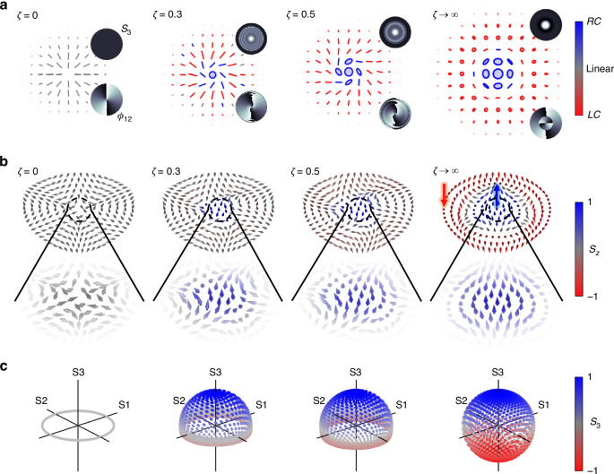 The alternative text for this image may have been generated using AI.
a A horizontally polarized LG mode (with ℓp = 1 and p = 0) incident on a q-plate, produces a vector mode with a radially polarized field pattern (in the near field) but carrying a net OAM charge of ℓp. Initially, the field contains zero spin density as it is populated by linear polarization states. On propagation, the beam shows a varying chirality and spin density (S3), shown via the polarization ellipses, at various propagation planes. These propagation planes are marked by the ratio ζ = z/zR, with ζ = 0 corresponding to the image plane. The spin density (S3, top panel) and the relative phase (ϕ12, bottom inset) are shown at each propagation plane. b Spin textured fields represented by spin unit vectors for the various corresponding propagation planes, with selected zoomed-in regions. Initially, the spin vectors point in the transverse plane, then gradually accumulate upward right-circular (RC) and downward left-circular (LC) spin components at the center and away from the origin, respectively. In the far field, there is a clear boundary that separates the LC and RC spin components, indicative of the Hall effect – orbit dependent spin separation. c The population of polarization states is shown at each plane on the Poincaré sphere. Initially, only the equator is covered at the waist plane, since the field contains only linear polarization states. Eventually, full coverage is shown, illustrating that the field evolves into a full Poincaré beam
The position-dependent amplitudes have been derived analytically for cases where an LG mode is incident on a phase element that imparts a phase of e±iΔℓϕ similar to the phases imparted by the q-plate. It has been shown that the LG mode profile evolves into an elegant Laguerre-Gaussian (eLG)49 mode or, equivalently, into a Hypergeometric Gaussian (HGG) mode50. In this article, we will use eLGs to represent the modes as they evolve, i.e. \({\mathrm{eLG}}_{{p}_{{\text{A}}({\text{B}})}}^{{\ell }_{{\text{A}}({\text{B}})}}\), with a topological charge of ℓA(B) = ℓp ± Δℓ and a radial index \({p}_{{\text{A}}({\text{B}})}=\frac{1}{2}(| {\ell }_{p}| -| {\ell }_{{\text{A}}({\text{B}})}| )\)49. These quantum numbers explicitly depend on the Pancharatnam index, ℓp. Therefore, the amplitude changes in the polarization components of the fields satisfying \({f}_{{\ell }_{{\rm{A}}({\rm{B}})}}(r,z)\equiv | {\rm{e}}{\rm{L}}{{\rm{G}}}_{{p}_{{\rm{A}}({\rm{B}})}}^{{\ell }_{{\rm{A}}({\rm{B}})}}(r,z)|\), are responsible for the observed polarization profile changes that in turn produce areas of chirality and longitudinal spin (i.e.: S3 ≠ 0) in the propagated fields. The angular spectrum (equivalently the farfield amplitude profile) of these modes has the form (see Supplementary Material for complete expression),
$$\begin{array}{ll}{\mathrm{eLG}}_{{p}_{{\rm{A}}({\rm{B}})}}^{{\ell }_{{\rm{A}}({\rm{B}})}}(\rho ,z\to \infty ) & \begin{array}{cl}\propto & {i}^{-{\ell }_{{\rm{A}}({\rm{B}})}}{\rho }^{| {\ell }_{{\rm{A}}({\rm{B}})}| }{L}_{{p}_{{\rm{A}}({\rm{B}})}}^{| {\ell }_{{\rm{A}}({\rm{B}})}| }[{\rho }^{2}]\end{array}\\ & \begin{array}{cl}\times & \exp (i{\ell }_{{\rm{A}}({\rm{B}})}\phi )\end{array}\end{array}$$
(7)
where ρ is the normalized radial (wavenumber) coordinate showing the explicit dependence on the radial term \({\rho }^{| {\ell }_{{\text{A}}({\text{B}})}| }={\rho }^{| {\ell }_{p}\pm \Delta \ell | }\) which controls the radial distribution of the modes (see Supplementary Material for more details about radial amplitude separation). Therefore, this radial factor is the source of the asymmetry in the spin components that can be observed in the transverse plane of the fields. In Fig. 2c, we map the fields onto the Poincaré sphere and show the population of polarization states across a field. Initially, the field at z = 0, maps onto a ring on the equator of the sphere because the field has no longitudinal spin components (S3 = 0). However, as the field propagates, gradual coverage over the sphere is achieved, indicating the emergence of a longitudinal spin component (S3 > 0) in the fields. Furthermore, because states near the origin have a higher intensity, only one half of the Poincaré sphere is covered first and other states are gradually populated as the beam propagates. Eventually, the farfield (z → ∞) is fully occupied by all possible spin states. This is observed taking into account that the intensity of the fields in the radial direction decreases, and nearly about 8% of the peak intensity is detected with a typical off-the-shelf CCD camera (Thorlab’s CS505MUP1) under the influence of stray light and shot noise in the detector (CCD). In the Supplementary Material, we show the case where the entire field intensity can be resolved completely, and find that full coverage is observed immediately upon propagation; however, we use the former to mirror experimental conditions.
Experimental validation
Next, we performed an experiment to validate the above (See experimental details in Methods). Horizontally polarized LG modes were prepared sequentially (using a spatial light modulator) with varying topological charges, ℓp ∈ {1, − 1, 2, − 2}, with each mode imaged onto a q-plate that transfers a net charge of ± Δℓ = ± 1 for each circular polarization component σ±, respectively. This produces our HyOP mode, carrying a Pancharatnam topological charge ℓp.
The Stokes parameters are shown in Fig. 3a at various propagation planes (ζ = {0, 0.3, 0.5, 0.7, farfield(ff)}) first for ℓp = 1, with the last row showing the relative phase ϕ12. Although the S1 and S2 Stokes parameters have the same number of lobes as shown in the two middle columns (second and third rows) of Fig. 3a, the only change observed is in the spiraling nature of the pattern upon propagation due to curvature and relative Gouy phase between the evolving field’s components. The twist of the spiral phase observed in the relative phase (ϕ12, last row of Fig. 3a) is seen to depend on the sign of the Pancharatnam topological charge during propagation. However, its handedness (direction of increasing phase in the azimuth direction) is preserved. On the other hand, the total beam intensity (S0) and spin densities (S3) are seen to change upon propagation as predicted, due to the amplitude change, with the left-handed CP component occupying the center. In contrast, the right-handed CP components dominate regions further away from the center.
Fig. 3: Experimental stokes parameter analysis.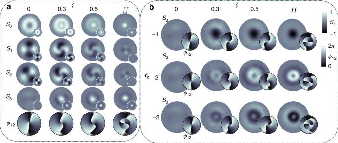 The alternative text for this image may have been generated using AI.
a Measured Stokes parameters, Sj, for ℓp = 1 at various propagation planes, labeled here as the ratio ζ = z/zR with ζ = 0 corresponding to the image plane. The last row shows the relative phases, ϕ12, showing a winding number 2Δℓ ≈ 2 for all propagation planes. b The measured z component of the Stokes parameter S3(r), characterizing the spin density of the field at different planes, ζ and the corresponding relative phase (ϕ12, see inset). This is shown for ℓp = − 1, 2 and − 2
Next, in Fig. 3b, we varied the input Pancharatnam topological charge (ℓp ∈ { − 1, 2, − 2}) and show the spin densities (S3) and the relative phases ϕ12. All the cases also exhibit identical relative phase profiles, although the spin densities (S3) differ, resulting in different amplitude responses. In contrast to ℓp = 1, ℓp = − 1, it produces a spin density profile, S3, that is inverted, showing that the chirality in the field has switched; now the right-handed CP amplitudes dominate in the center, whereas the left-handed CP components dominate at a distance away from the center. For ℓp = ± 2, we also see the same trend where the dominant polarization switches depending on the input topological charge. Further, the magnitude of the input charge (ℓp) is seen to control the radial profile of the spin density (S3) owing to the radial modes that emerge in the field upon propagation, since the field components become eLG modes that have regions of nonoverlapping intensities. Moreover, for ℓp = ± 2, a vortex is observed since both circular polarization components have non-zero OAM after passing through the q-plate, which can also be inferred from the S3 components. We emphasize that the same q-plate was used to obtain these results, indicating that the local chirality is primarily attributed to the presence of Pancharatnam topological charge in the fields.
The sphere coverage and polarization (ellipse) profiles at different propagation planes are depicted in Fig. 4. The polarization ellipses are represented in terms of handedness, with red indicating left-handed CP and blue representing right-handed CP.
Fig. 4: Observing orbit induced spin generation upon propagation.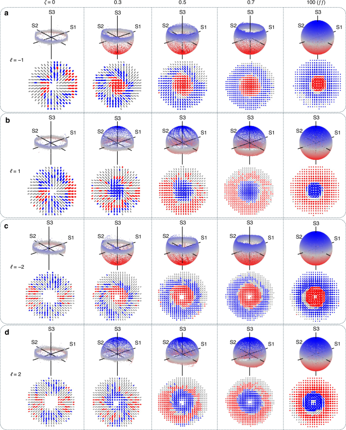 The alternative text for this image may have been generated using AI.
Reconstructed Poincaré sphere coverage and polarization ellipses for Pancharatnam topological indices (a) ℓp = − 1 and (b) ℓp = 1 at various propagation planes (ζ = z/zR). The same plots are shown for topological charges (c) ℓp = − 2 and (d) ℓp = 2, illustrating the emergence of spin from a vectorial field that initially has zero spin density in the paraxial regime
Results were obtained for positive topological charge ℓp > 0 (rows b and d of Fig. 4), resulting in right-handed CP at the origin of the field. Conversely, for ℓp < 0 (rows a and c of Fig. 4), left-handed CP was observed at the center/origin of the field. We observe that the fields only contain linearly polarized states at the plane of the q-plate, as expected, since only linear polarizations are observed, indicated by the population of the fields on the equator of the Poincaré sphere. This can be inferred from the radially oriented linear polarization states, indicating that S3 ≈ 0. The presence of a few observed ellipses at this plane can be attributed to experimental errors induced by the waveplates. This can be improved through careful calibration of the waveplates. As we observe propagation, circular polarizations begin to form, indicating an increase in the spin density of the field. For ℓp = 1( − 1), the accumulation of elliptical polarization states is also seen through the occupation of states beyond the equator. In fact, the polarization states initially dominate the top half of the sphere, since the LC (RC) components have a larger amplitude contribution and eventually cover the whole sphere once the beam approaches the farfield. Similarly, this is observed for ℓp = ± 2, however, the structure has a characteristic vortex at the center.
Topology-driven optical Hall effect
Lastly, in Fig. 5, we show the measured farfield spin textures for each of the HyOP modes having different Pancharatnam topological charges. In these illustrations, it can be seen that for ℓp = 0 all the spin vectors lie in the transverse plane, showing that there is no spin separation. However, once ℓp ≠ 0, the separation of RC and LC components is observed, confirming the topologically driven nature of the spin separation in the optical field, which only depends on ℓp. Therefore, the initial Pancharatnam topological charge, which characterizes the net OAM of the modes, induces transverse spin currents analogous to an electric field that induces similar currents in a magnetic system. The spin currents can be measured from \(\overline{J}=\langle \frac{\partial {S}_{3}}{\partial y},-\frac{\partial {S}_{3}}{\partial x}\rangle\). We show this for our experimental results in the insert of Fig. 5, demonstrating an azimuthal spin current in each case. This is because of the radial spin gradient seen in the S3 components of the field with an abrupt switch in helicity observed in each case. In fact, more generally, this Hall effect can be interpreted as a spin-orbit Hall effect arising from the spatial separation of spin and orbital angular momentum components in vector vortex beams during propagation. For example, the inner and outer rings of Fig. 4c in the ff possess an azimuthal phase of \(\exp (i\phi )\) and \(\exp (i3\phi )\), respectively. Although we have not directly measured the OAM content of each polarization component, the fact that their regions do not overlap suggests that each mode may contribute an OAM density confined to its respective nonoverlapping area. Finally, it is important to emphasize that spin and optical chirality in these beams are local properties. Due to the divergence of the full three-dimensional integrals, the (integral) total values of the spin and optical chirality for beams are instead expressed in terms of their linear densities, i.e., the corresponding quantities per unit length along the z-axis: ∝ ∫S3dr⊥ = 0. Clearly upon free-space propagation of the radially polarized field the integral values are conserved.
Fig. 5: Emergent orbit-induced Hall effect.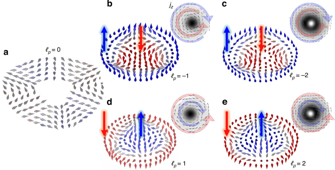 The alternative text for this image may have been generated using AI.
Experimental spin textures of the farfield modes for Pancharatnam topological charge ℓp = 0, − 1, − 2, 1, 2 in panels (a)-(e), respectively, illustrating an orbit-induced Hall effect. The transverse spin separation is visualized by the spin-current insets, which reveal an azimuthal flow that reverses direction as it approaches the field’s origin. This behavior shows that the polarization handedness is well-defined near the center and changes beyond a certain radial distance, indicative of an optical spin-Hall effect. The insets show the spin currents (\(\overline{J}\)) which reveal the azimuthal spin currents due to the spin-Hall effect